Optimization
Decisions are made based on preferences. Either it is to minimize the monthly expense for a person living with a tight budget or to maximize the revenue of a restaurant for a business owner, we need to consider our preference or criteria (minimize or maximize) to form a solution. This process is called optimization and optimizing based on a preference is an objective. When we only focus on single objectives, we can easily sort out the best solution. However, in reality, we frequently need to take multiple objectives into consideration. And more than often, the objectives we want to optimize are conflicting each other. For example, when a car has the most comfortability and the best performance, we know it is going to cost a fortune on the fuel. In order to solve these multi-objectives optimization problems, we can consider the Pareto front.
Pareto Dominance and Pareto Front
Assume that there is a set of solutions for a scenario where our objective is to maximize X and minimize Y. These solutions are illustrated by the graph below where each point represents one of the available solutions. We can see that in general, solutions with a higher X value also have a higher Y value. In another word, our objectives (maximizing X and minimizing Y) are conflicting each other.
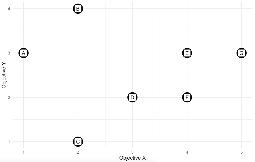
If we look at solution A and C, we can see that solution C has a lower Y value and a higher X value. And thus, solution C is more preferable to A. The same can be said to solution F compared to solution E. Although both solutions have the same X value, but solution F has a lower Y value and thus we prefer solution F to E. When a solution is no worse than the other one in any perspective and it is strictly better from at least one perspective, then we say this solution dominates the other, or the other solution is dominated by this solution. In our example, solution C dominates A and solution F dominates E. Solution A and E are dominated solutions. Meanwhile, we can’t make the same conclusion about solution F. By observation, no other solution dominates solution F. Solution G has a higher X value, but it also has a higher Y value and solution D has a lower Y value, but it also has a lower X value. Since we can’t improve either X or Y without hurting the others, we say solution F is non-dominated. All non-dominated solutions form the set of Pareto front.
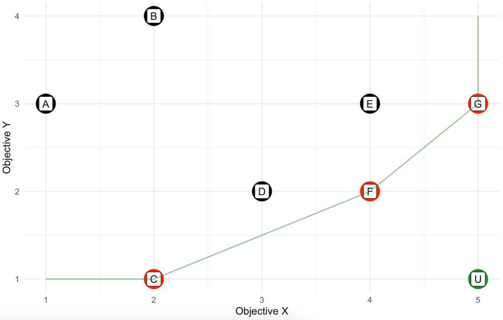
From our example, we notice that the Pareto front consists of solution C, F, and G. Any other solution is dominated by at least one of the solutions in Pareto front and solutions in the Pareto front are non-dominated solutions. If we connect the Pareto front solutions, we can get a visual representation of the Pareto front formed by the given solution. Any solution that lies on this line will be non-dominate solution. For aesthetic reason, we extend the Pareto front to both ends so that it covers the full range.
Utopian point and optimal solution
Pareto front helps us to narrow down the solutions to a few that we must make a trade-off in choose one over the other. Is there a mechanism to identify one single best solution among the Pareto front solutions? Assume that we can take the X and Y values from each individual solution apart and combine with X and Y values from the other solutions, the best solution we could get under the assumption is called the utopian point. As the name suggest, it is unrealistic. But it provides a good reference on how far away each Pareto front solution is from this ideal solution.
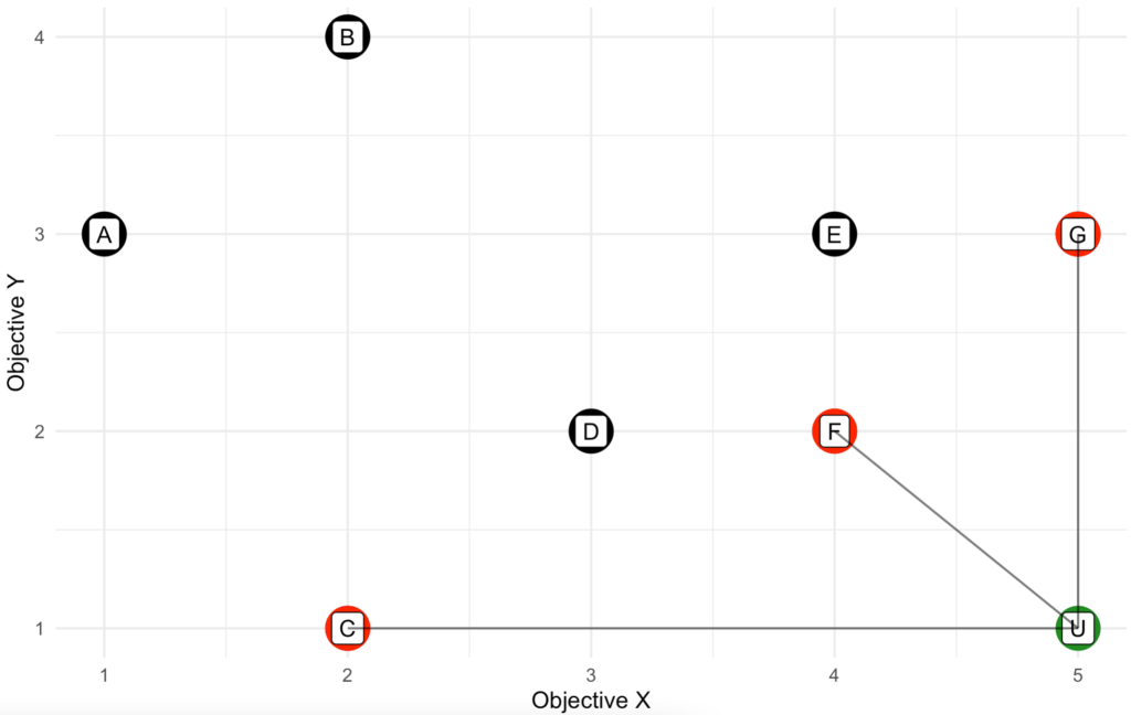
Since we view each preference (either X or Y) equally important, we can measure the distance from each of the Pareto front solution to the utopian point. The one with the shortest distance is the optimal solution. It makes sense because the solution closest to the ideal solution is either balanced across both X and Y, or one of them is so close to the best possible value we can get, and it compensates the other value that is worse off.
Get the optimal solution on d3VIEW
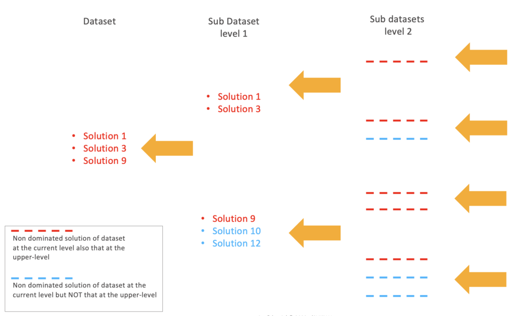
As demonstrated above, in order to find all Pareto front solutions, we need to compare all solutions to make sure that no one dominates the candidate for the Pareto front solutions. This can be computationally expensive. In d3VIEW, we adopt the Kung’s method[1]. First, we sort the first objective from the most optimal to least optimal. Then, we divide the dataset into two (top half and bottom half), find the non-dominated solutions in each sub dataset, and combine them. The set of non-dominated solutions from the top half sub dataset will still be non-dominated for the whole dataset. However, this is not the case for those from the bottom half sub dataset. Then, we check if any of the non-dominated solutions from the bottom half is dominated by any non-dominated solutions from the top half. After identifying all non-dominated solutions, we combine all the non-dominated solutions from the two sub datasets. Recursively, we can find all non-dominated solutions of the given dataset with fewer efforts.
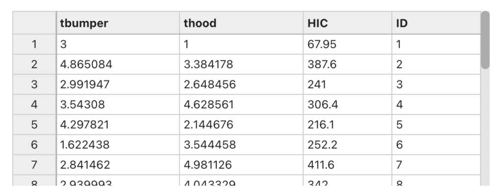
Here is an example of Pareto optimization using a sample HIC dataset. Each row of the dataset represents a solution to the problem. And we are interested in a solution that has the min value for all three variables “tbumper”, “thood”, and “HIC”.
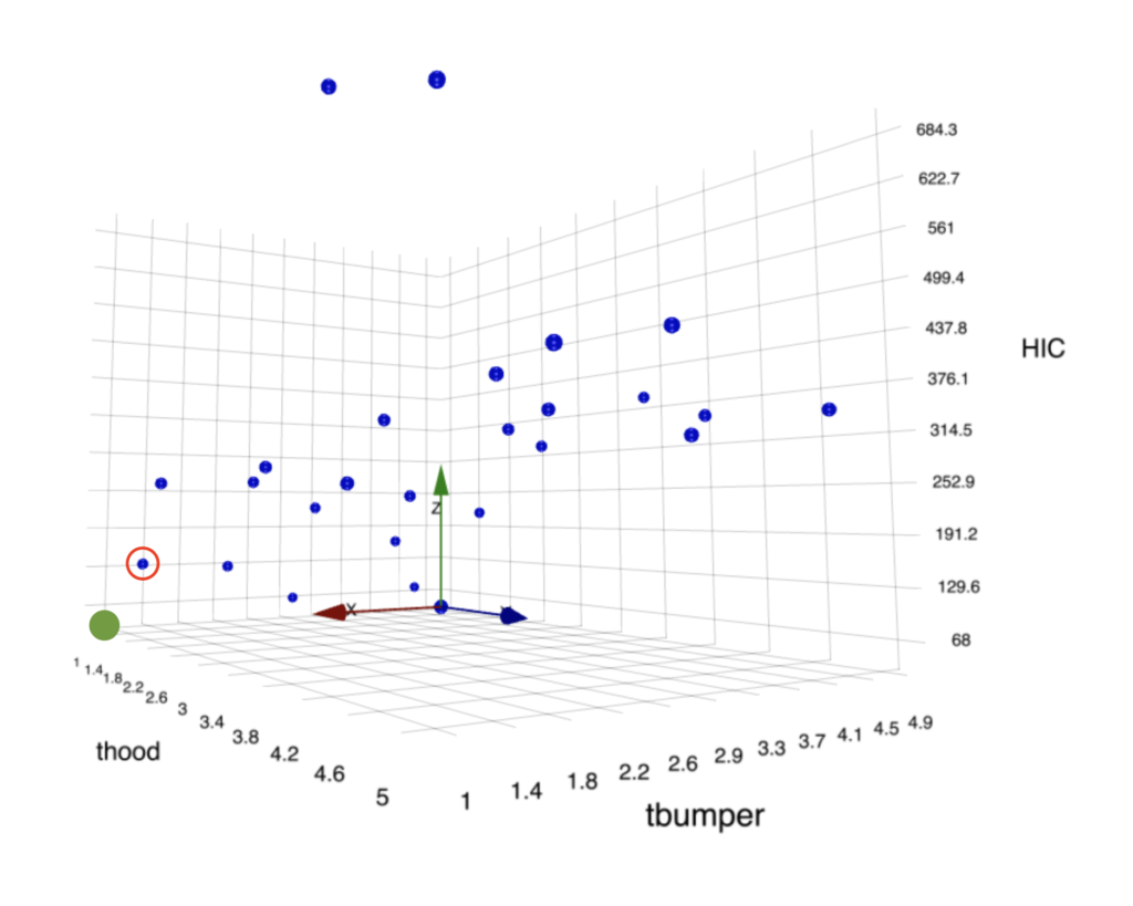
By providing this dataset to the “Dataset Compute Pareto Front Optimal” worker on d3VIEW, in return, we get the optimal solution in the output.

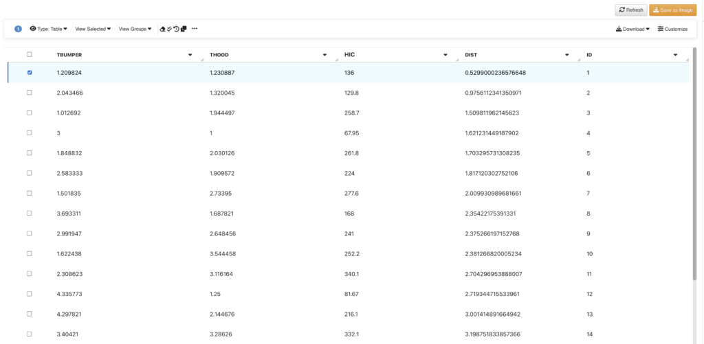
Or we can provide this dataset to the worker “Dataset Compute Pareto Front Sorter” and it will return all the points with the distance information sorted in ascending order, which means, the first point we see on the top is the optimal solution.
Reference
[1] H. T. Kung, F. Luccio, and F. P. Preparata. 1975. On Finding the Maxima of a Set of Vectors. J. ACM 22, 4 (Oct. 1975), 469–476. https://doi.org/10.1145/321906.321910