12. Parallelization¶

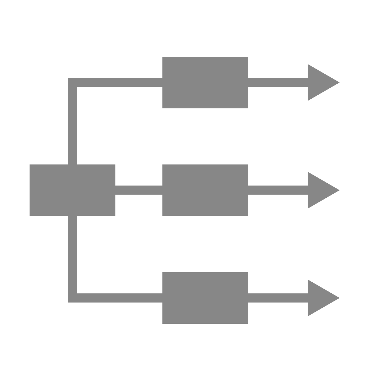
Parallelization is a process by which you can run multiple workers in parallel execution. It is primarily helpful in speeding up the execution or to run multiple simulations at the same time. Attached is the image of three simulations run in parallel.

^{Parallelization}

Easily create a parallelization of a section of a workflow by using the select multiple option and right-clicking.

Click on the Select Multiple option at the bottom right corner. Then, we’ll drag-select the part of the workflow that we want to clone. Finally, we’ll right-click and choose the “Clone” option. Finish by connected the cloned parts to the start and end workers.

12.1. Machine Learning Parallelization¶

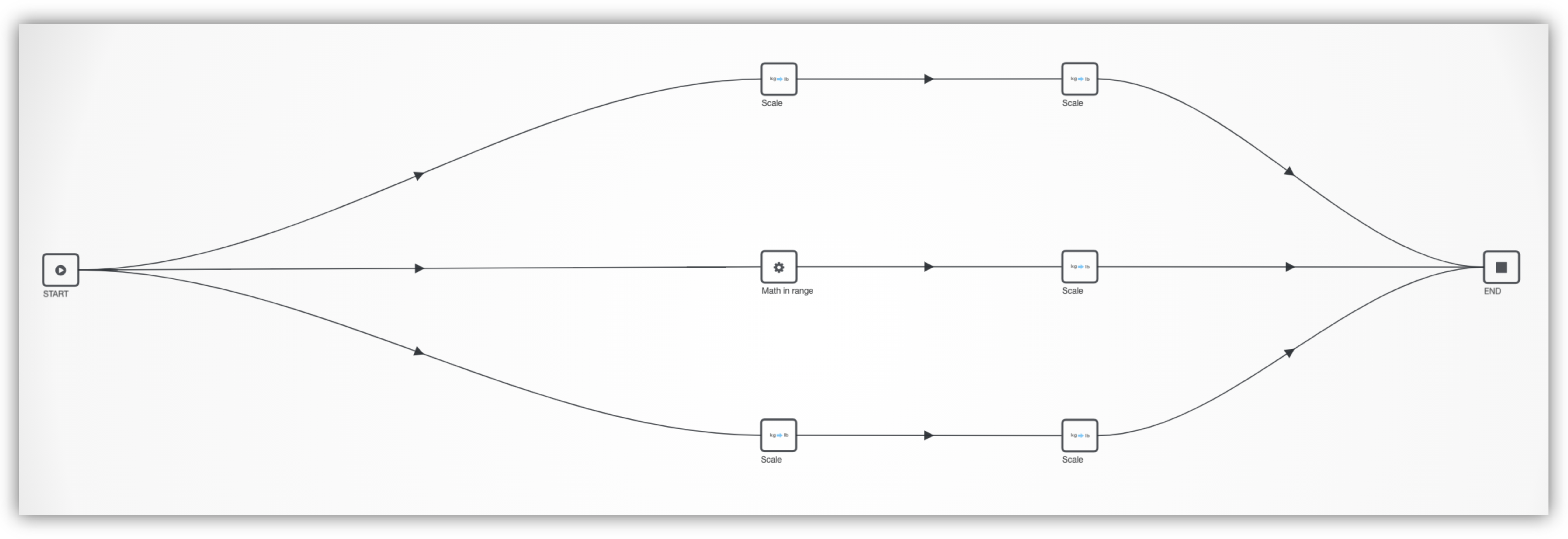
As mentioned before, parallelizing workflows allows us to run similar processes simultaneously, reducing time and increasing efficiency. We can even do this with ML models, allowing us to predict targets in different ways at the same time. In this section, we’ll review a parallelized machine learning workflow for based on spotweld specimen datasets for normal, bending and shear.

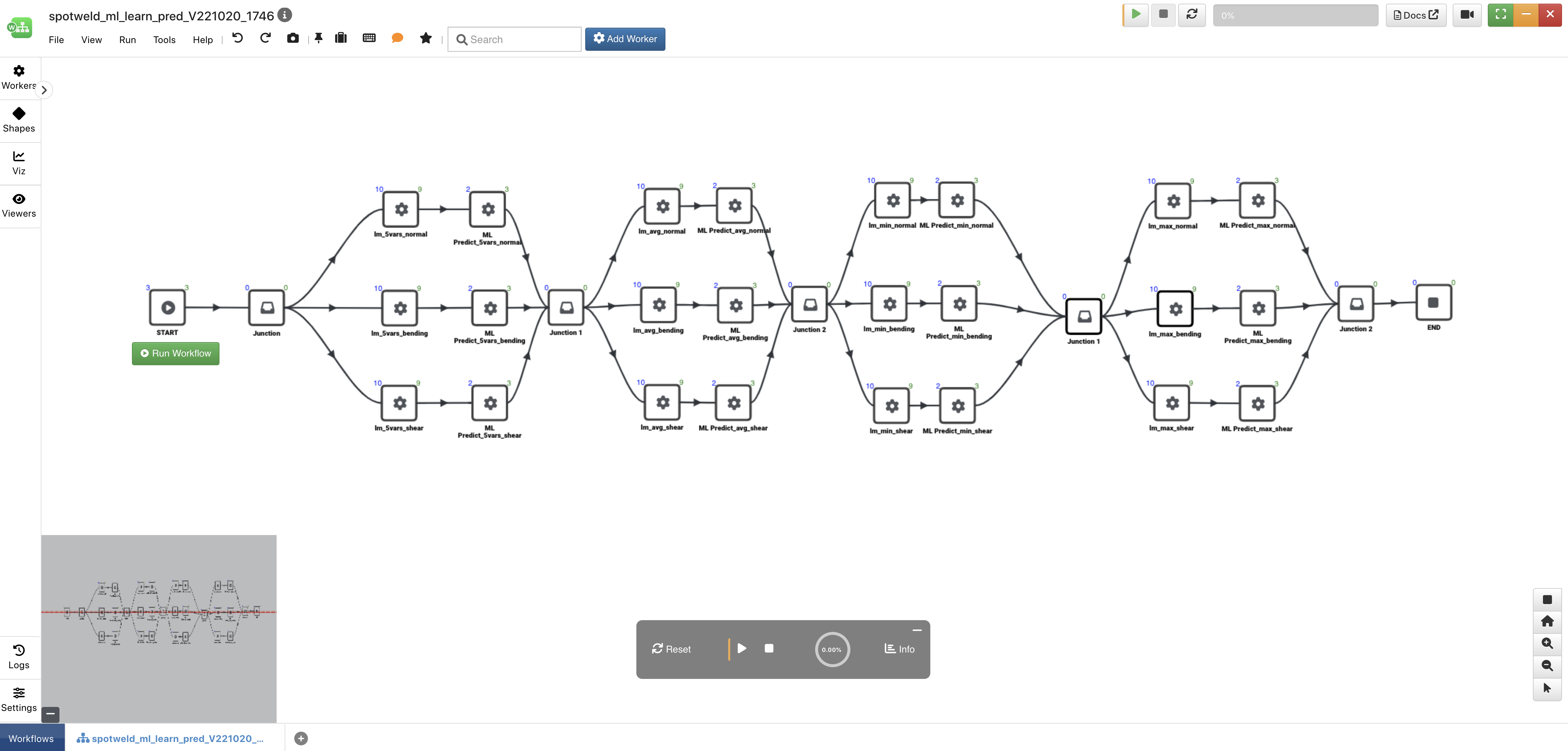
^{Figure 1: Spotweld Parallelized Machine Learning Workflow}

Workers¶

The three workers used in this workflow, aside from the START and END workers, are *ML_LEARN_LINEAR, *ML_PREDICT and the Edge Junction (in shapes). *ML_LEARN_LINEAR will be our Machine Learning model using Linear Regression. *ML_PREDICT will be how we predict our target column based on the above model. The Edge Junction is used as a connection point between our four groups of models. This is not necessary but helps us see the distinction between the groups. (More on groups in the next section)

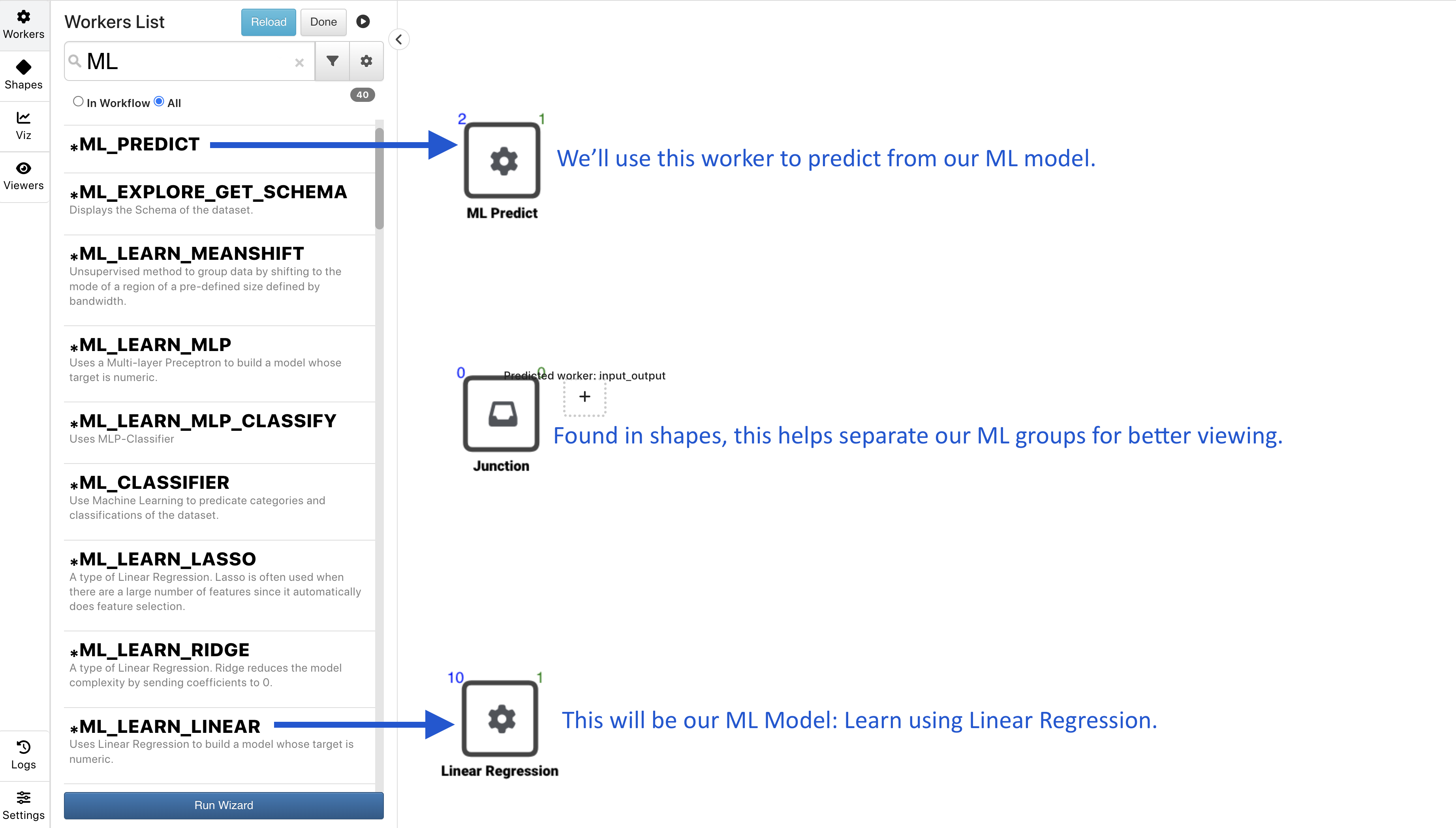
^{Figure 2: ML Workers}

Machine Learning Models¶

The following image maps our where we are using the *ML_LEARN_LINEAR workers in the workflow.

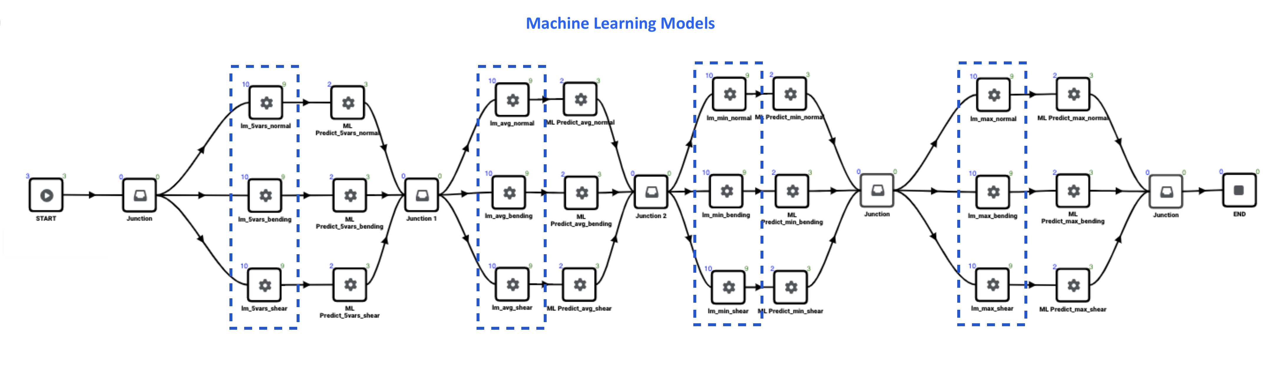
^{Figure 3: Machine Learning Models}

Machine Learning Predictions¶

The following image maps our where we are using the *ML_PREDICT workers in the workflow.

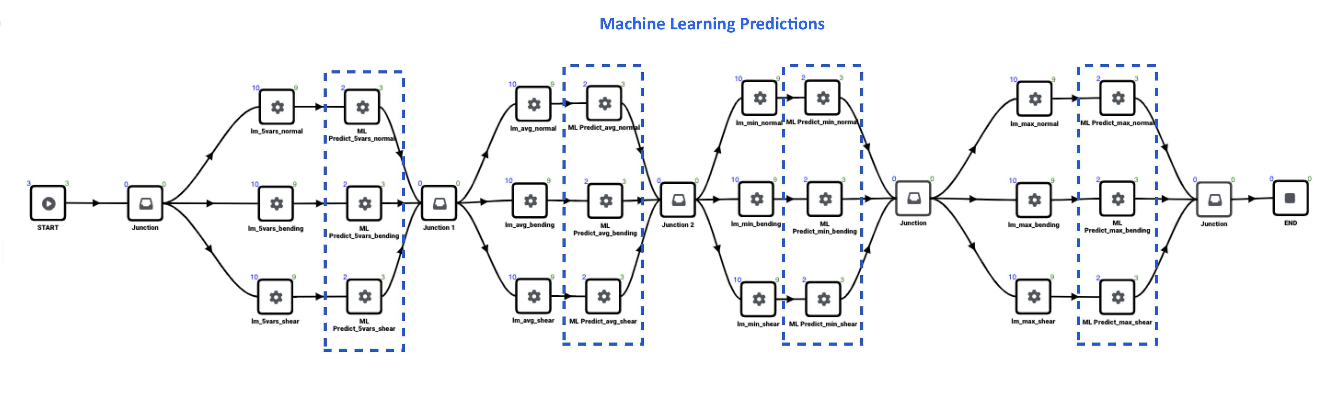
^{Figure 4: Machine Learning Predictions}

Groups and Types¶

As mentioned before, the workflow is sectioned into four different groups. Each group has different input features for predicting our target columns (normal_stress_madeup, bending_stress_madeup and shear_stress_madeup).

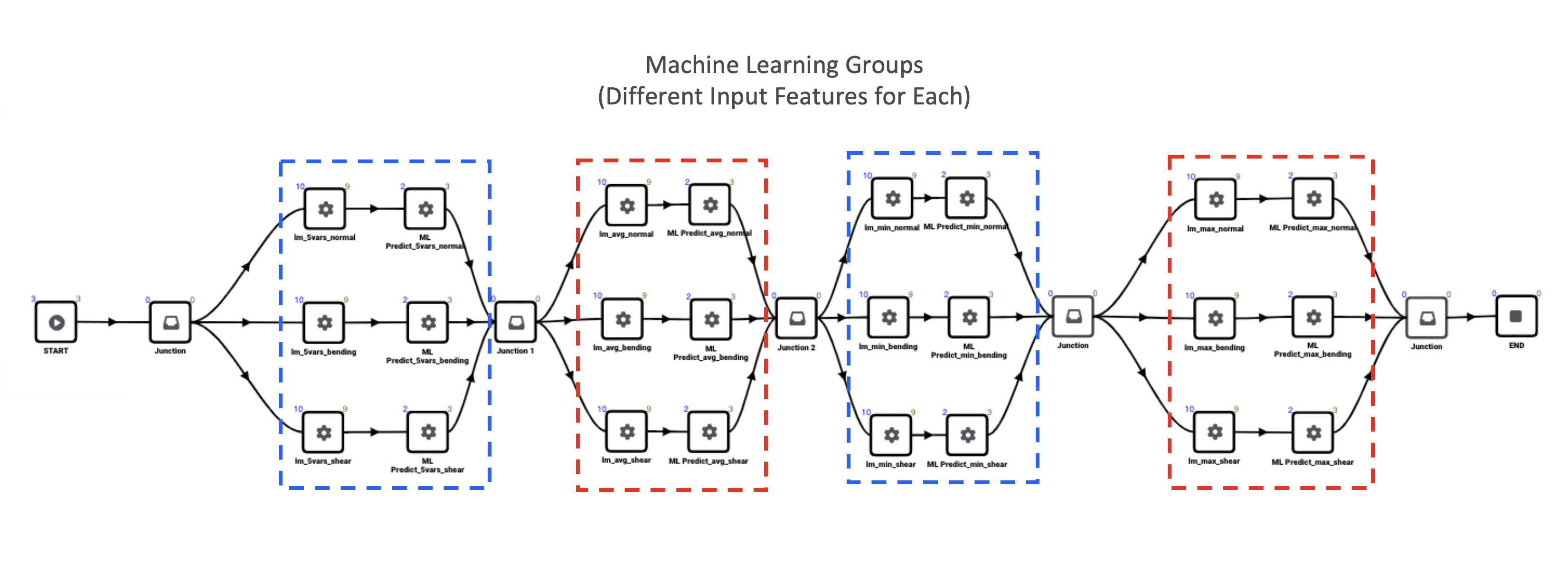
^{Figure 4: ML Groups}

There are three spotweld datasets we are using for our ML models: normal, bending and shear. The following images map out where we are modeling and predicting for each type.

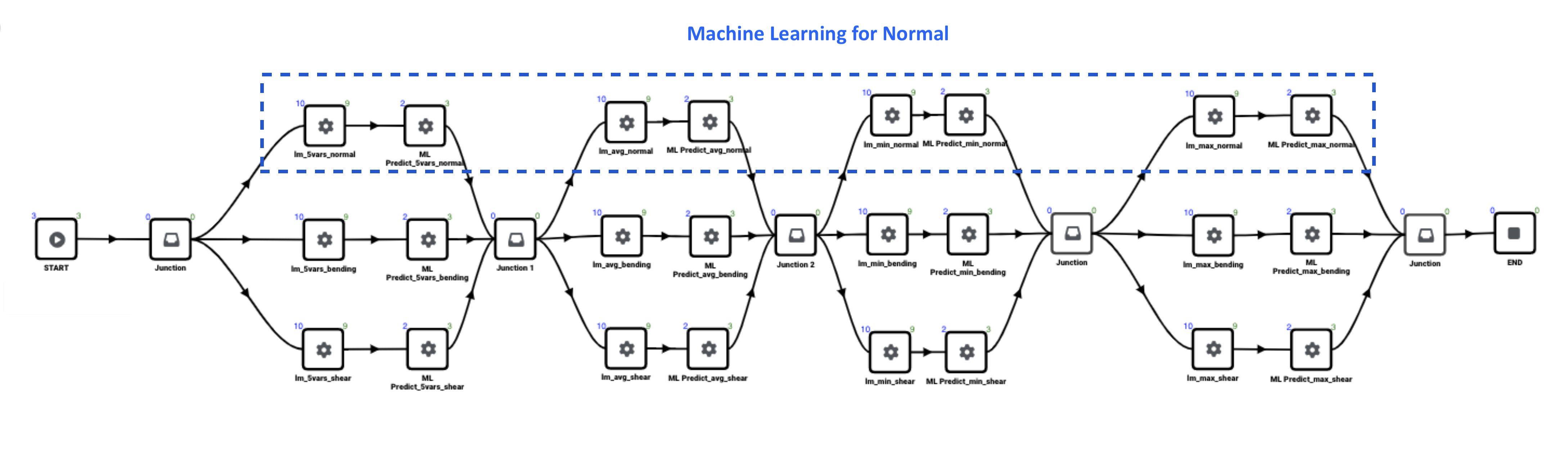
^{Figure 5: Machine Learning Normal}

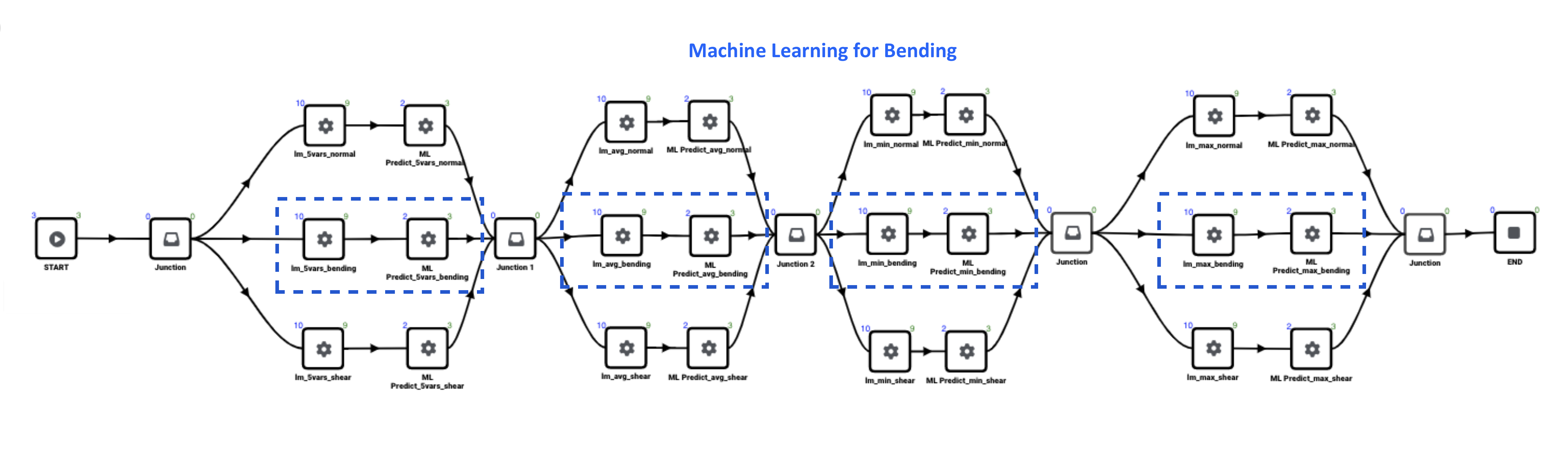
^{Figure 6: Machine Learning Bending}

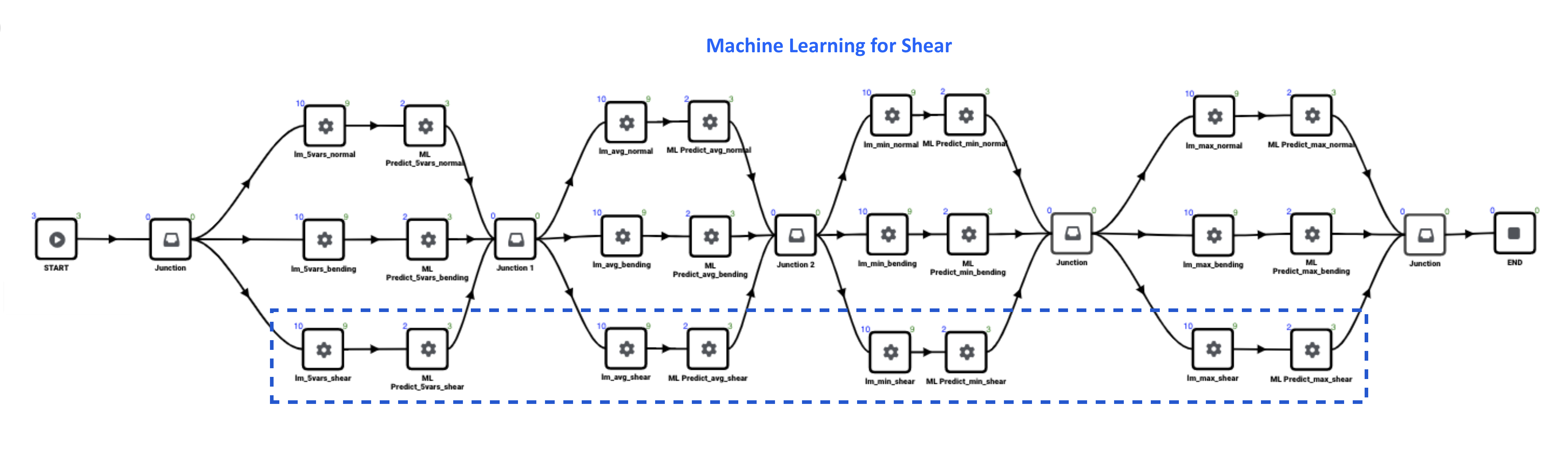
^{Figure 7: Machine Learning Shear}

Input Features and Target Columns¶

All three ML models within a group have the same input features. The following image maps out the input features for each group.

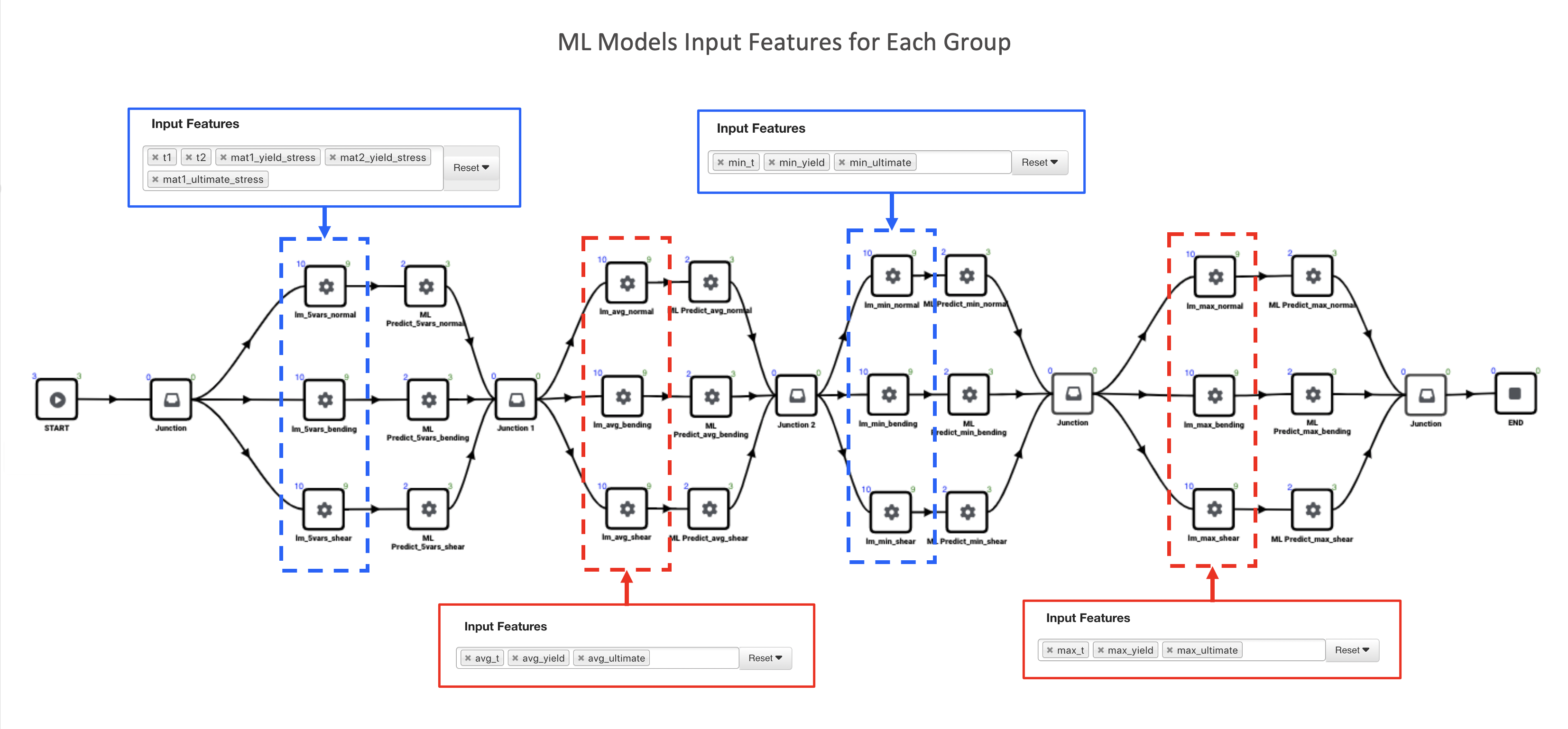
^{Figure 8: Input Features}

For the target column, each model uses “stress_madeup”, named according to the spotweld type (normal_stress_madeup, bending_stress_madeup and shear_stress_madeup) as illustrated in the following image.

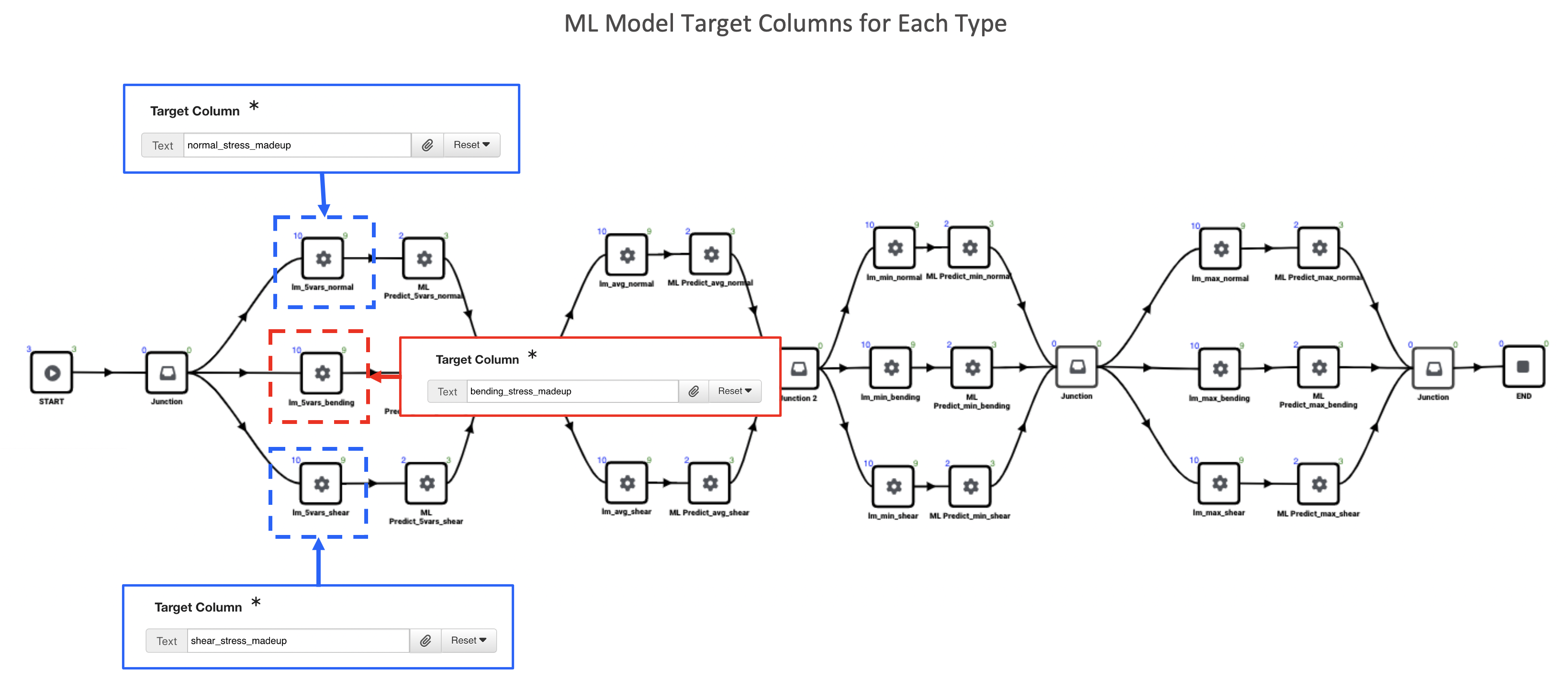
^{Figure 9: Target Columns}

Worker Configurations and Outputs¶

Let’s review how the machine learning workers are configured along with the outputs by mapping out an example for each.

*ML_LEARN_LINEAR¶

The following images map out the first group of ML model workers for each type. The only different between these configurations and the other groups is the Input Features. Refer back to the section above to see the different Input Features for each group.

The Normal model uses the corresponding dataset and target column. Click on View Simlytiks next to an output to visualize it.

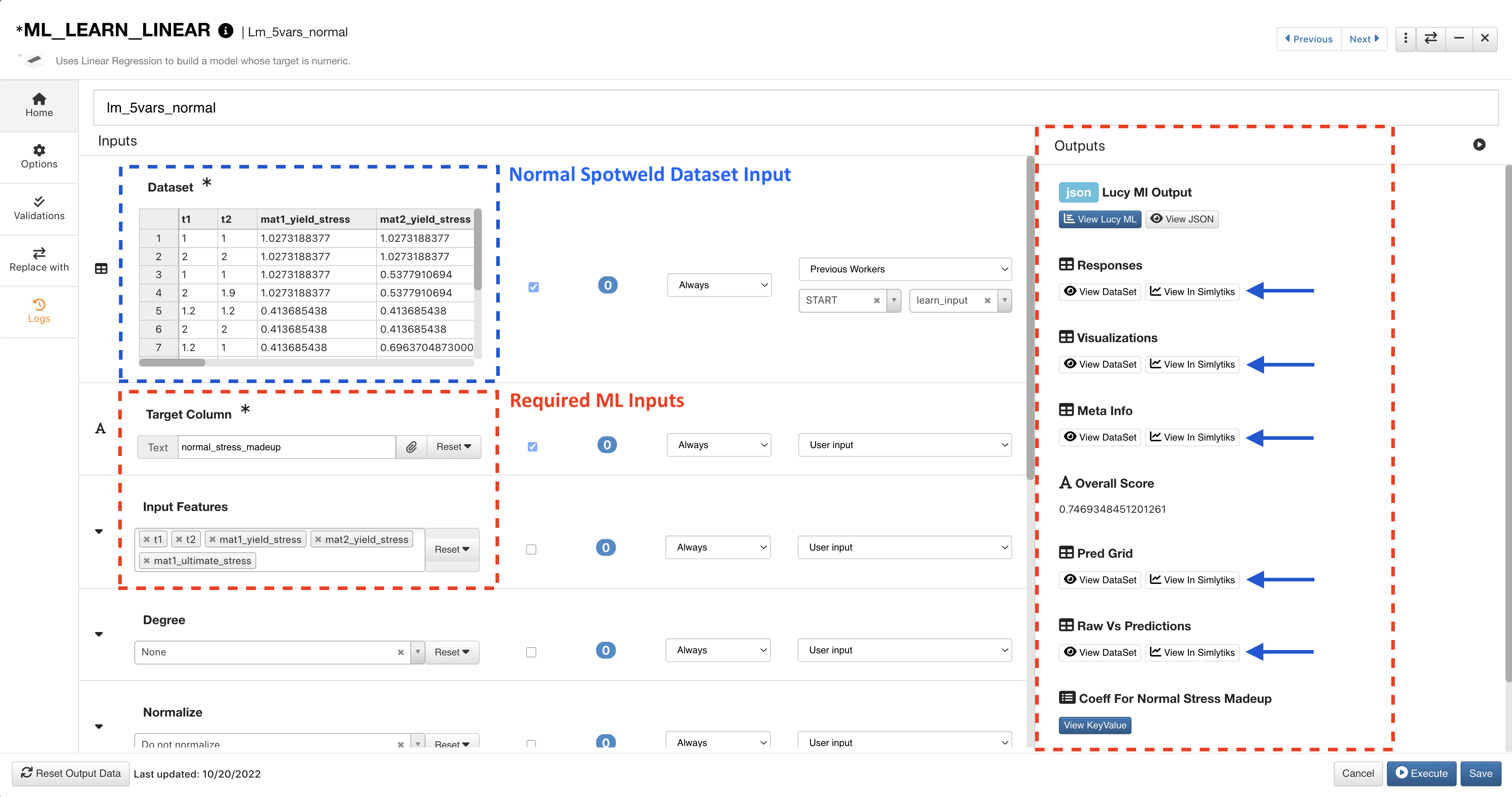
^{Figure 10: ML Learn Normal}

The Bending model uses the corresponding dataset and target column. Click on View Simlytiks next to an output to visualize it.

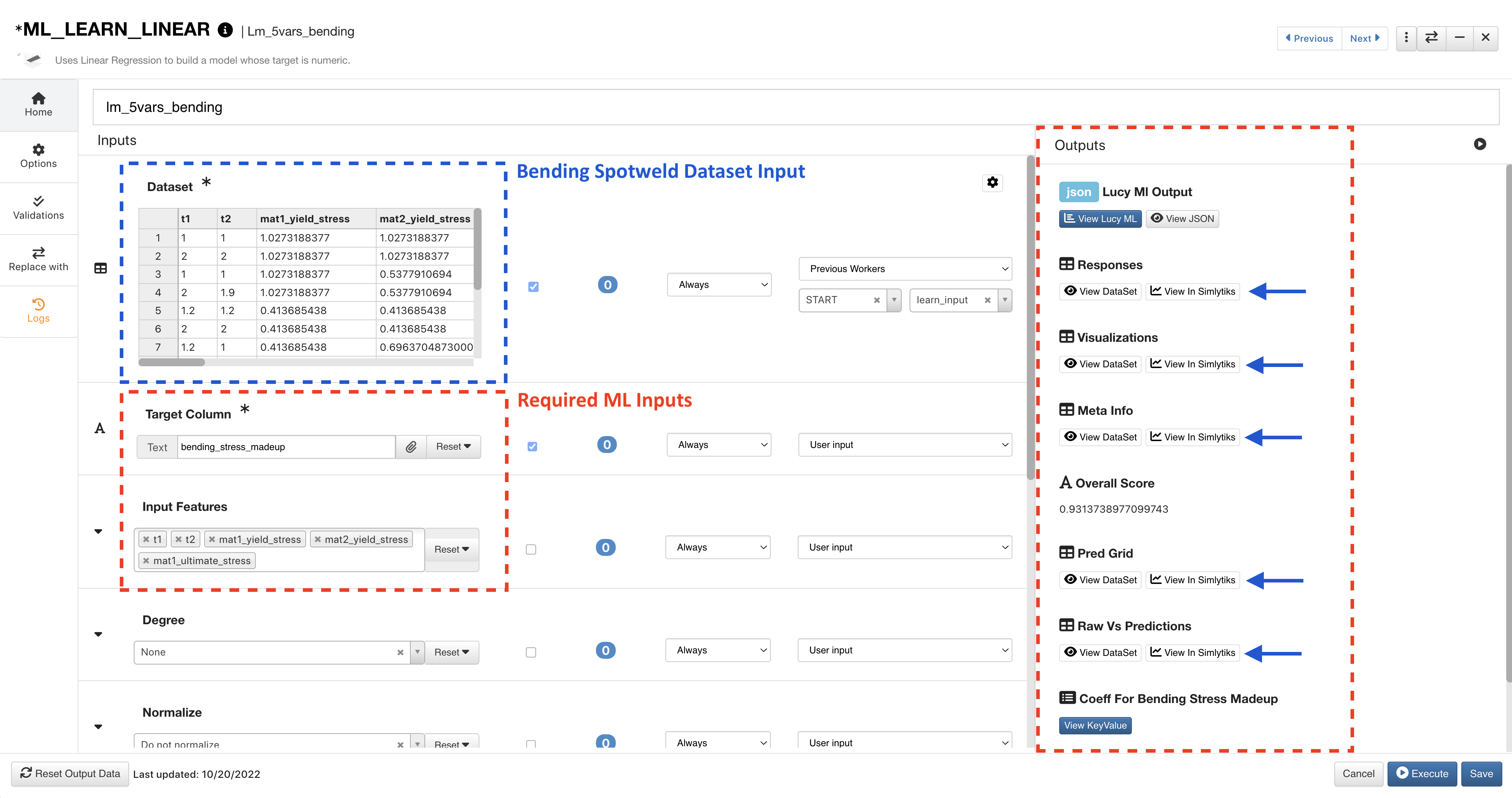
^{Figure 11: ML Learn Bending}

The Shear model uses the corresponding dataset and target column. Click on View Simlytiks next to an output to visualize it.

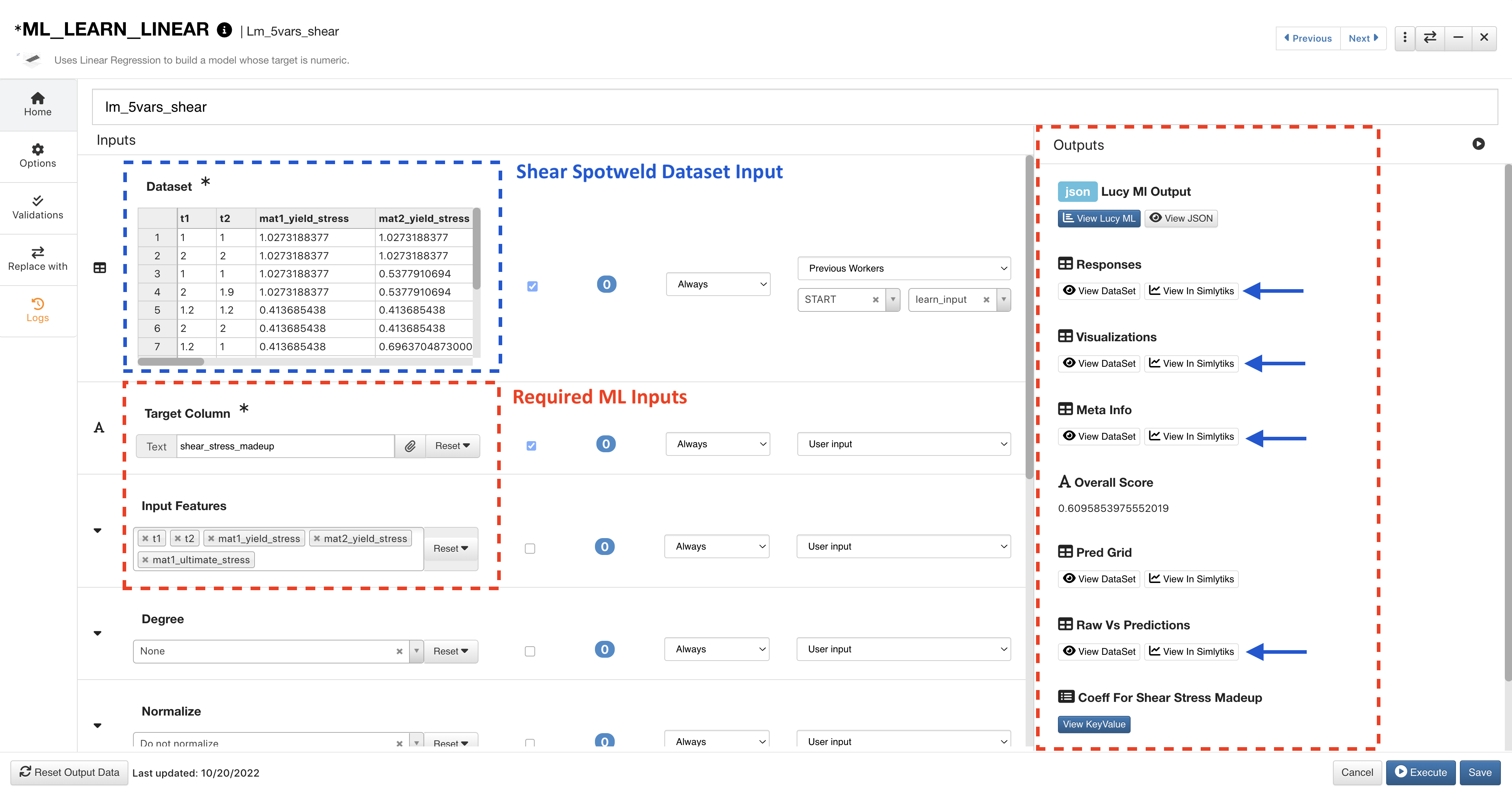
^{Figure 12: ML Learn Shear}

*ML_PREDICT¶

The following images map out the first group of ML Predict workers for each type. The only different between these configurations and the other groups is which Model Path output we are using. This output will be the corresponding previous worker output for the particular type (normal, bending, shear).

The Normal prediction uses the corresponding dataset and ML model path output from the previous worker. Click on View Simlytiks next to an output to visualize it.

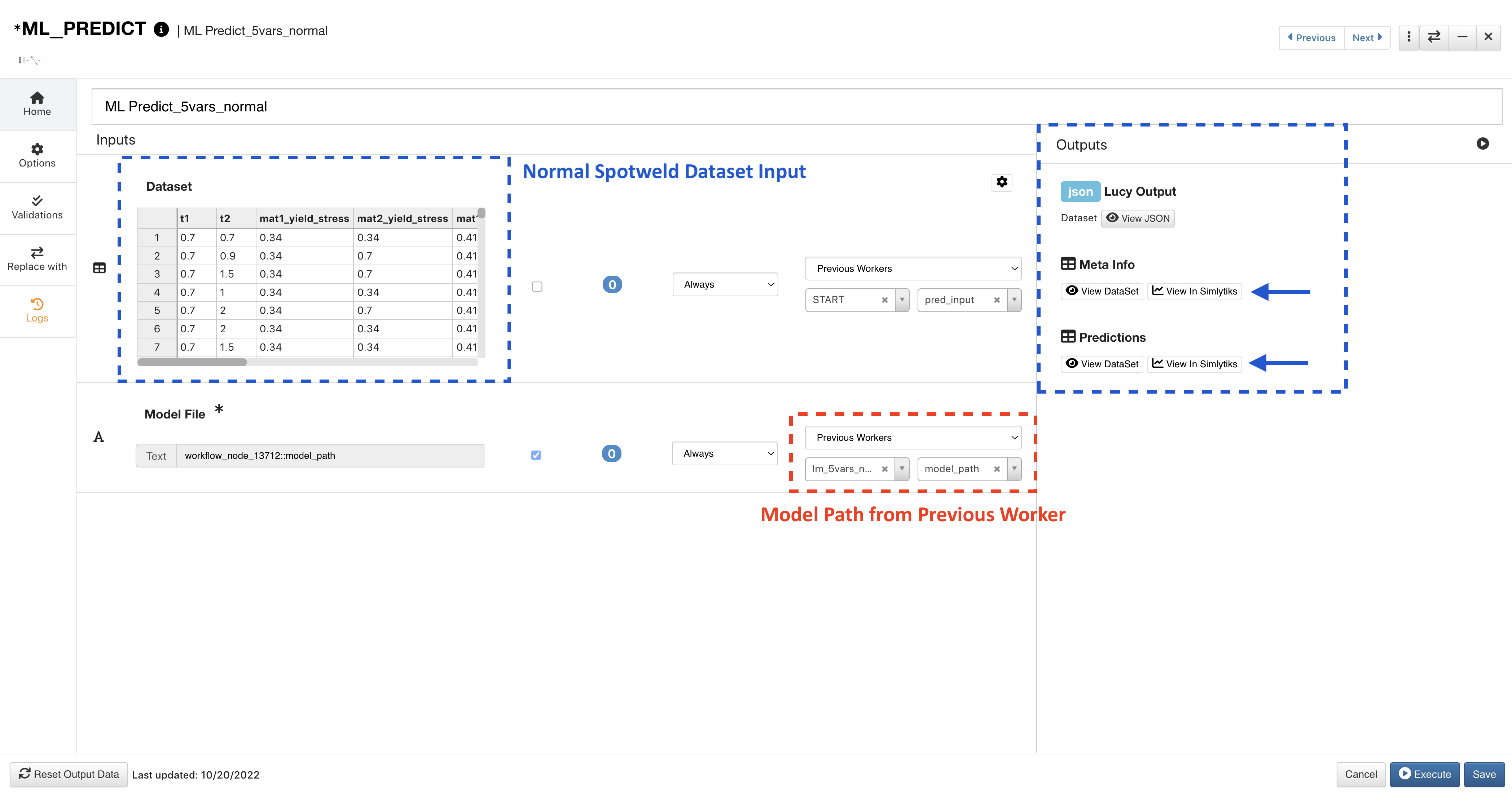
^{Figure 13: ML Predict Normal}

The Bending prediction uses the corresponding dataset and ML model path output from the previous worker. Click on View Simlytiks next to an output to visualize it.

^{Figure 14: ML Predict Bending}

The Shear prediction uses the corresponding dataset and ML model path output from the previous worker. Click on View Simlytiks next to an output to visualize it.

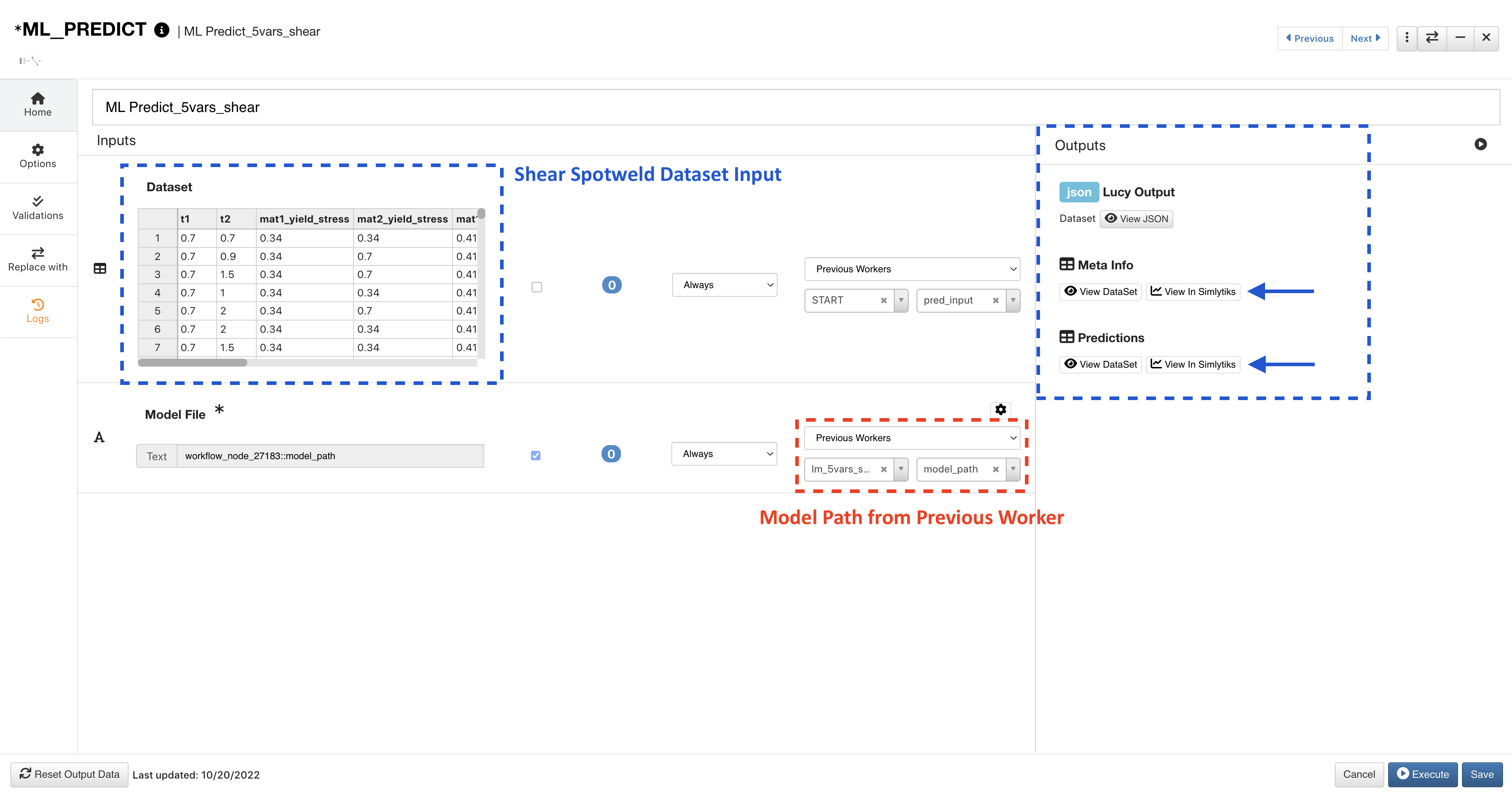
^{Figure 15: ML Predict Shear}