32. Peacock 3D
Conventional 2D exploration has its limitations which is why d3VIEW incorporates a 3D application called Peacock to help examine and explore models in 3D space. This application integrates most prominently with simulations and Simlytiks and can be used to unravel more information from our 3D models. Watch the following video for an overview of the application’s capabilities:
What Will Be Covered
- Extracting and uploading models
- Understanding the interface
- Advanced features
- Exporting and sharing
32.1. Extracting and Uploading
There are two ways we can use Peacock for exploring our models. First, we can extract 3D files from a simulation or physical test. Second, we can upload our own 3D files under a simulation or physical test to open in Peacock. Let’s first go over what files are supported in Peacock.
Supported Files
Peacock 3D supports a range of 3D files including extracted simulation files:
| Name | Extension | d3VIEW Generated Only |
|---|---|---|
| Peacock3D | .js3d | X |
| Peacock3D | .js3d.zip | X |
| Stereolithography (CAD) | .stl | |
| Polygon | .ply | |
| Object | .obj | |
| Visualization Toolkit | .vtk | |
| VTK Surface Models | .vtp |
Extracting 3D Models From Data
Let’s go over how to extract a 3D file for viewing in Peacock. We’ll be reviewing how to extract from a simulation, but we can also extract from physical test data so long as we have the data to support it.
After submitting a simulation (learn how to do that here), we’ll open it and go to the the responses page (1) (learn how to navigate simulations here) and click “Extract Responses” (2) to get started.
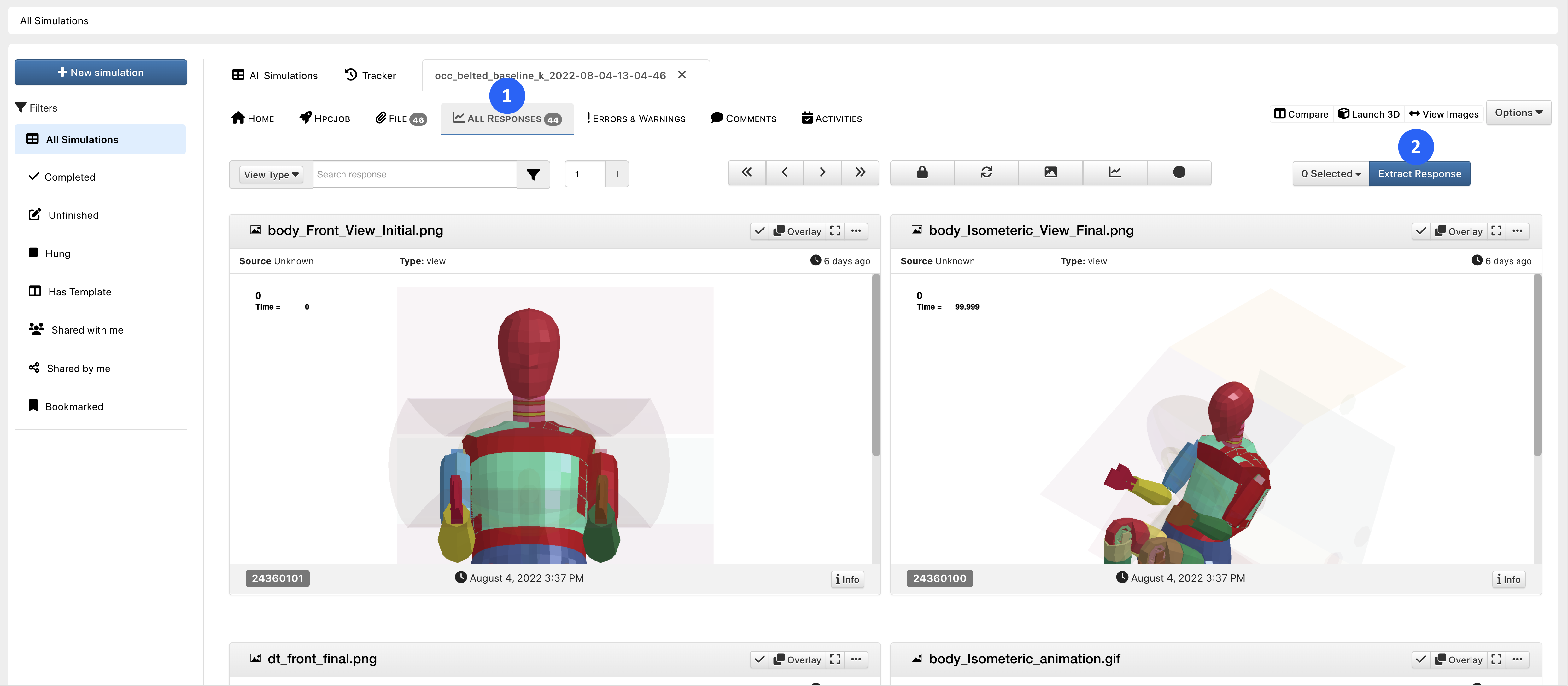
Figure 1: Simulation Responses Page
Once we have the Extract Responses window up, we’ll navigate to the dyna_d3plot Data source tab.
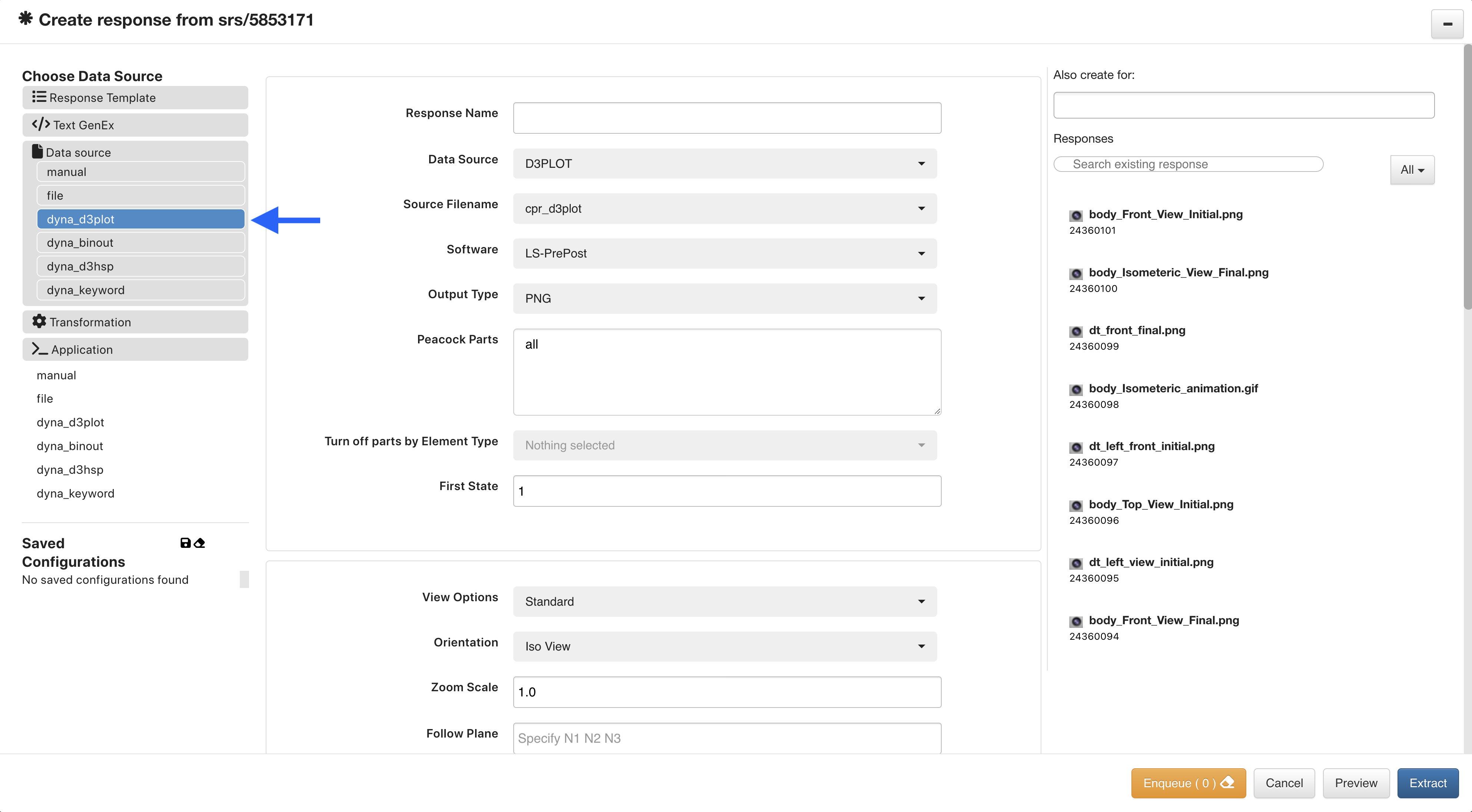
Figure 2: Extract dyna_d3plot Response
For this example, we are extracting from an occupant belted sample simulation (email support@d3view.com to get this simulation file). We’ll set up the parameters as follows making sure we name our model with the correct .js3d.zip extension, choosing Peacock3D as the output type and specifying a final state:
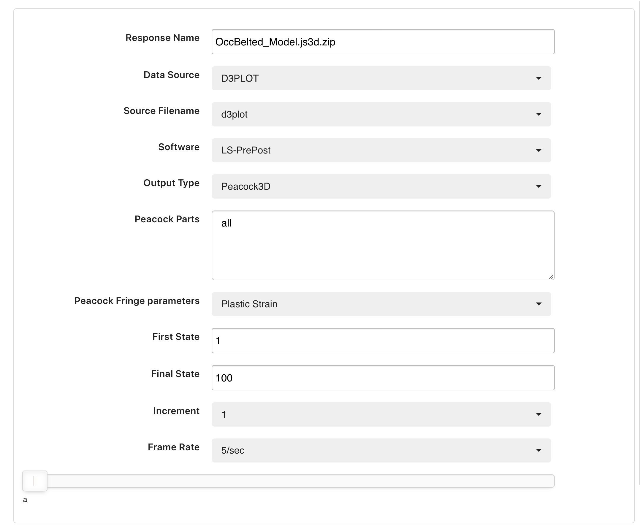
Figure 3: Extract dyna_d3plot Input Parameters
We can choose to preview the response first (1) and then go ahead and extract it (2).
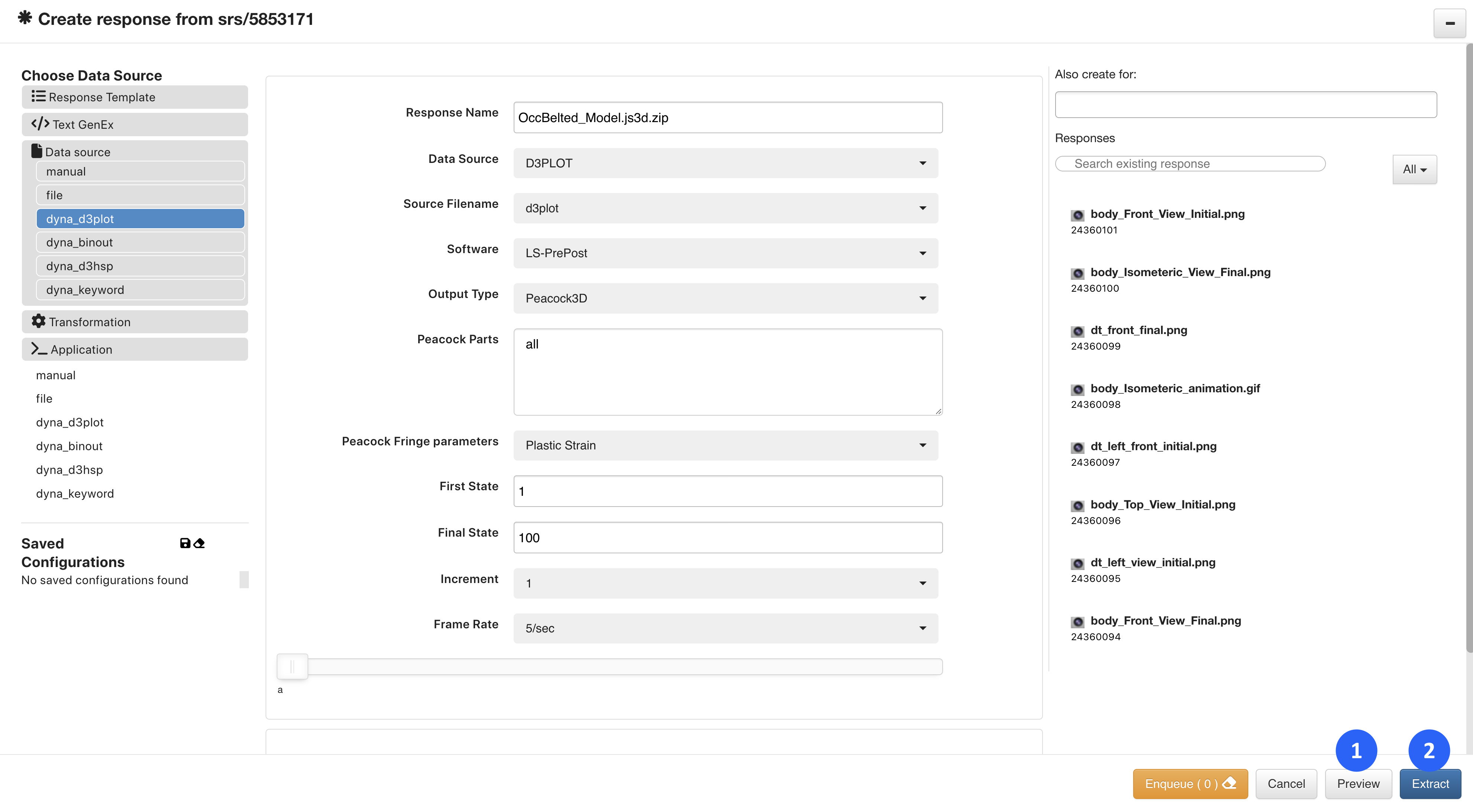
Figure 4: Extract Peacock 3D Model
After hitting extract, we should see our new response at the top of our simulation responses page. We’ll click on it and expand the window to start exploring it in Peacock.
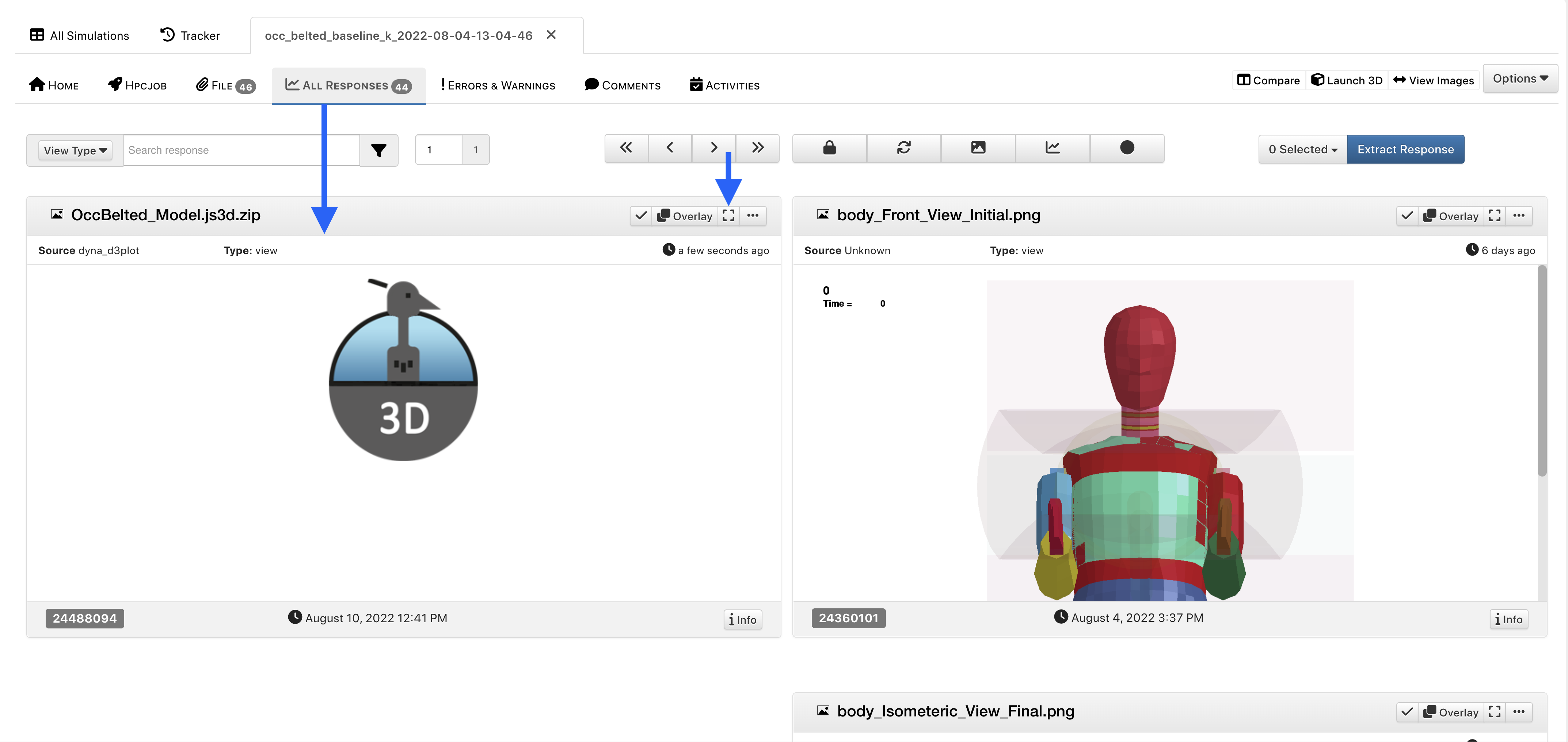
Figure 5: Extracted Peacock 3D Model
Uploading a Local Model
To upload a local 3D model, go to the Physical Tests application and upload your model as a new test (learn how to create a physical test in more detail here). In this example, we are uploading a brain PLY file and naming the test according. We’ll process the text to upload it to the platform.
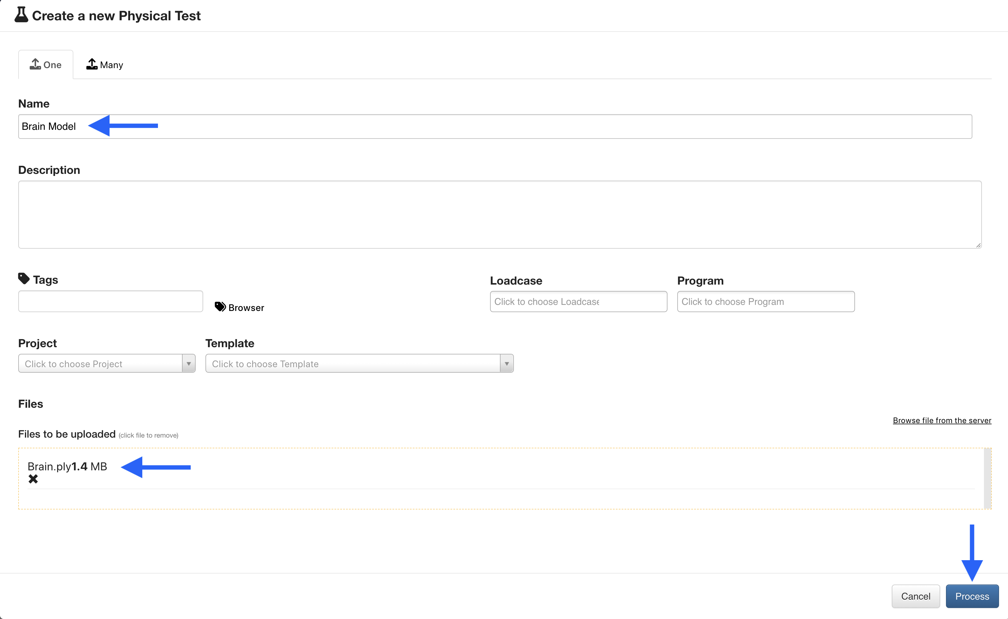
Figure 6: Upload Model as a Physical Test
The new test will show up on our Physical Tests main page. (Click the refresh button at the top if you don’t see it initially). We’ll click on its name to open it in a new tab.
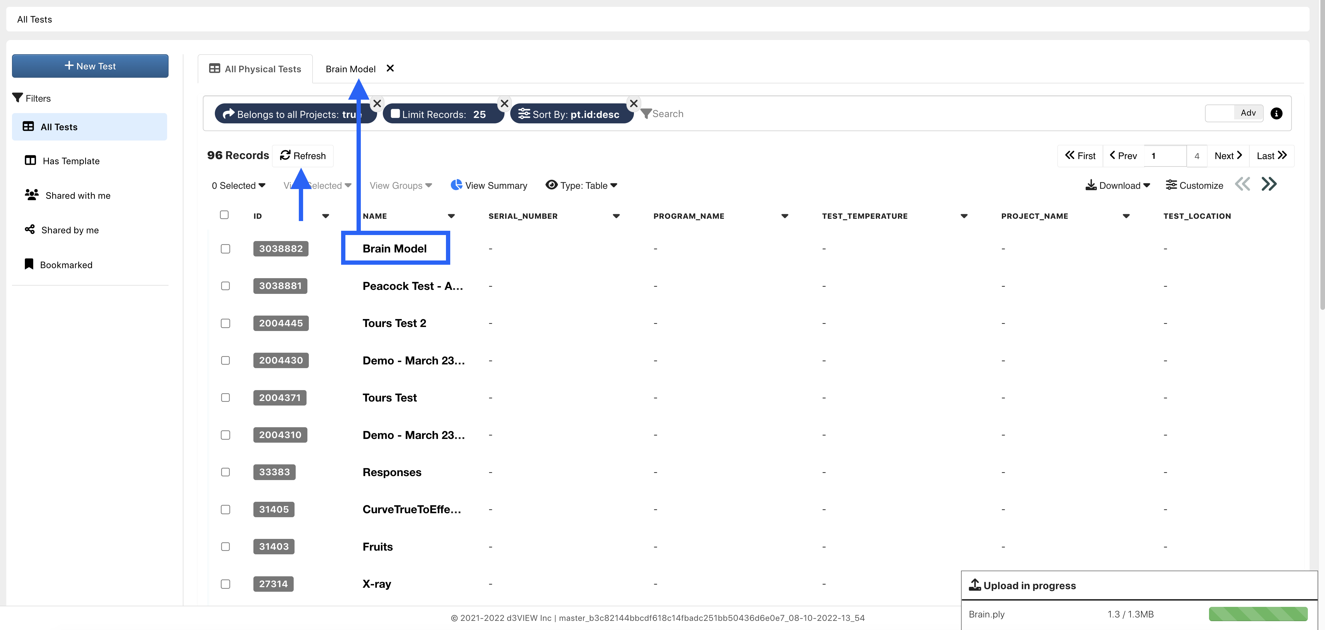
Figure 7: Open Physical Test Model
Under the Files section of the test, we’ll see our uploaded model.
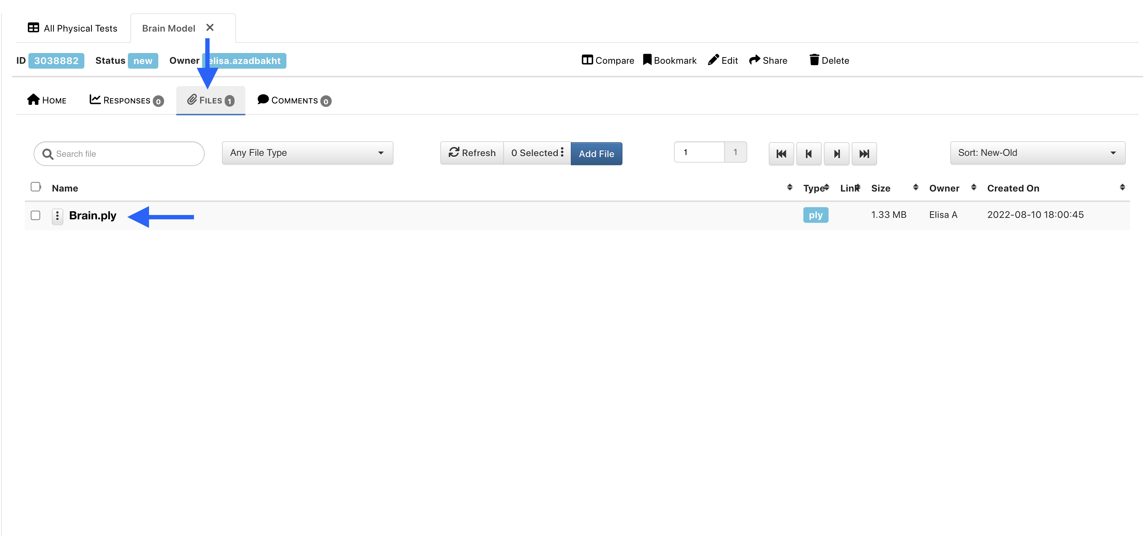
Figure 8: Model File
We can then click on the model name to open in a new Peacock window as shown in the following video:
Progressive Loading
When we upload and open large models, Peacock initiates progressive loading based on groups by user-defined parts list. This allows us to interact with intricate models sooner than waiting for the full model to load.
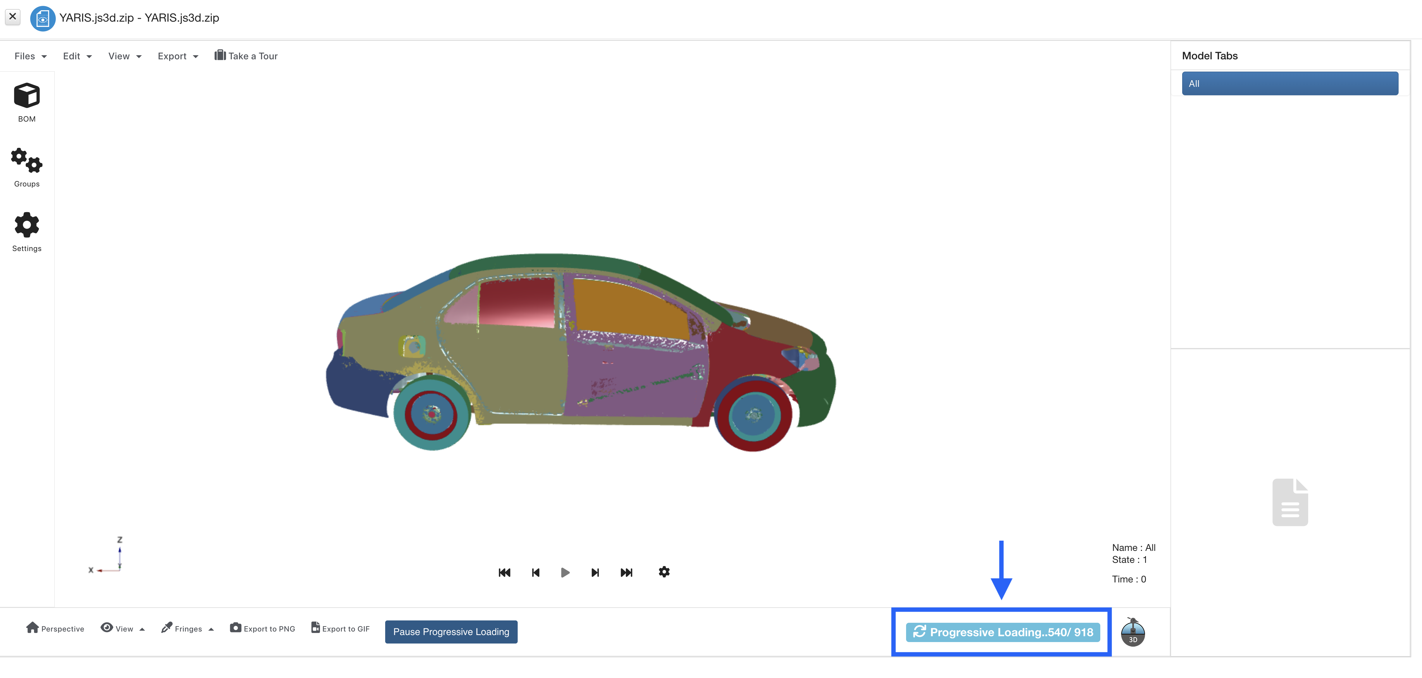
Figure 9: Progressive Loading
When we open a model of this caliber, we’ll see a progressive loading bar on the bottom right (1) and a Pause Progressive Loading button on the bottom left (2).
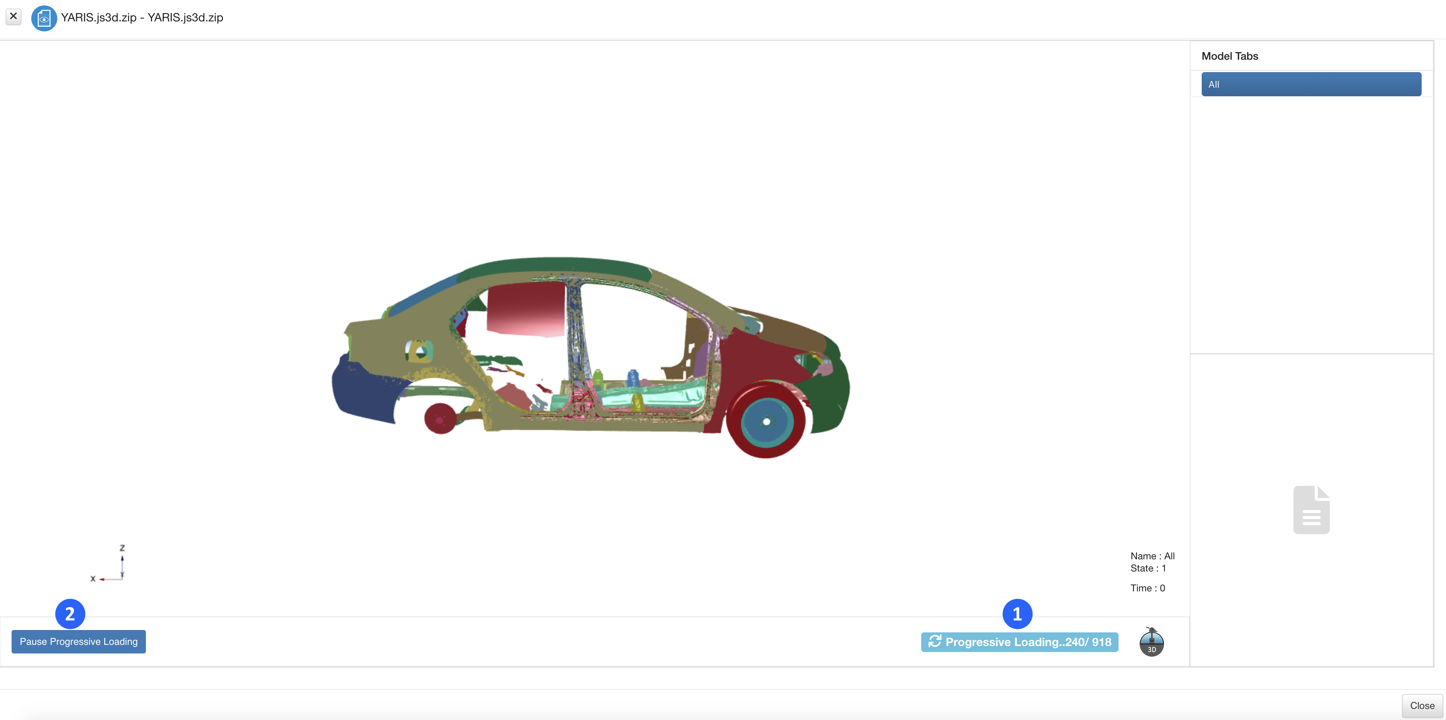
Figure 10: Progressive Loading Bar and Pause Button
Once we click pause, we’ll be able to interact with the semi-loaded model. We can see under the BOM, or Bill of Materials, menu (more on that here) which parts/groups have fully rendered, indicated with a green dot, and which still have yet to render, indicated with a red dot.
We can restart the rendering process by clicking the blue button again which will now say Play Progressive Loading.
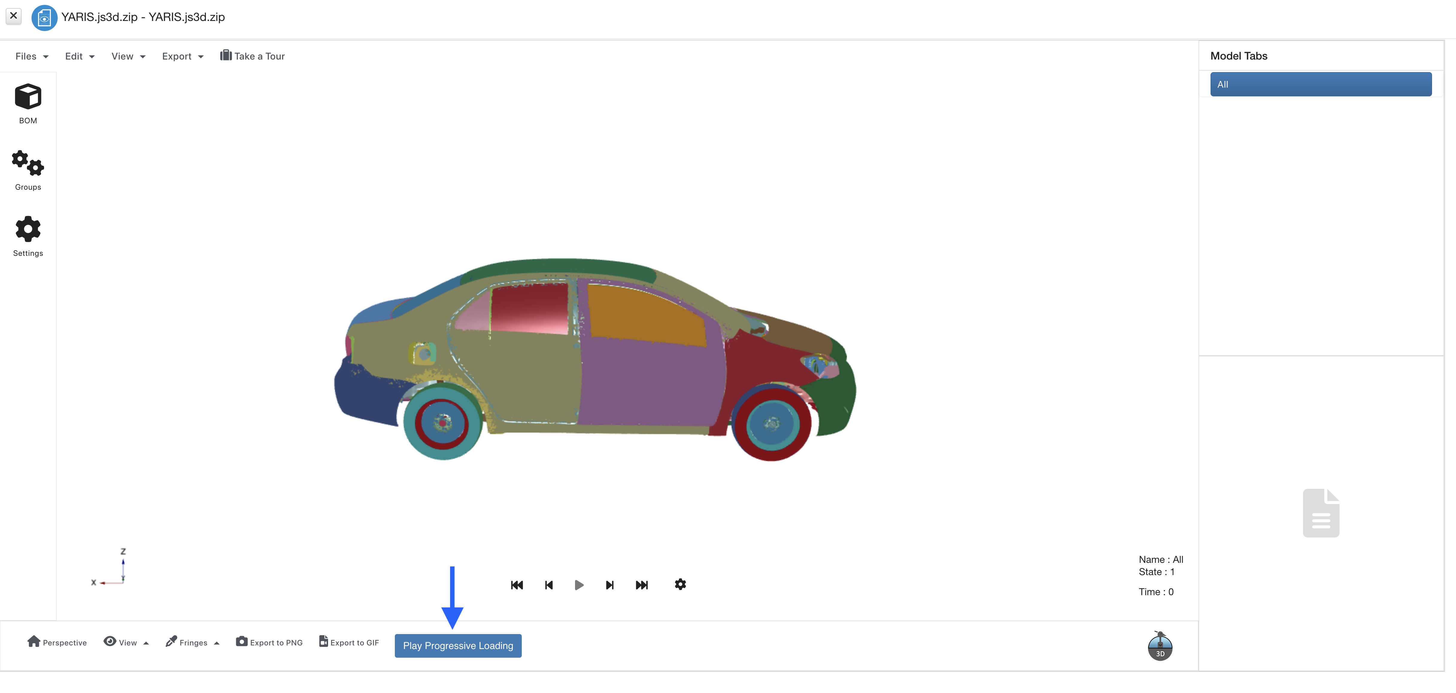
Figure 11: Play Progressive Loading
32.2. Navigation
In this section, we’ll go over the basics of how to navigate and explore a 3D model.
Peacock Interface
The following image maps the options available in the 3D app with descriptions for each below:
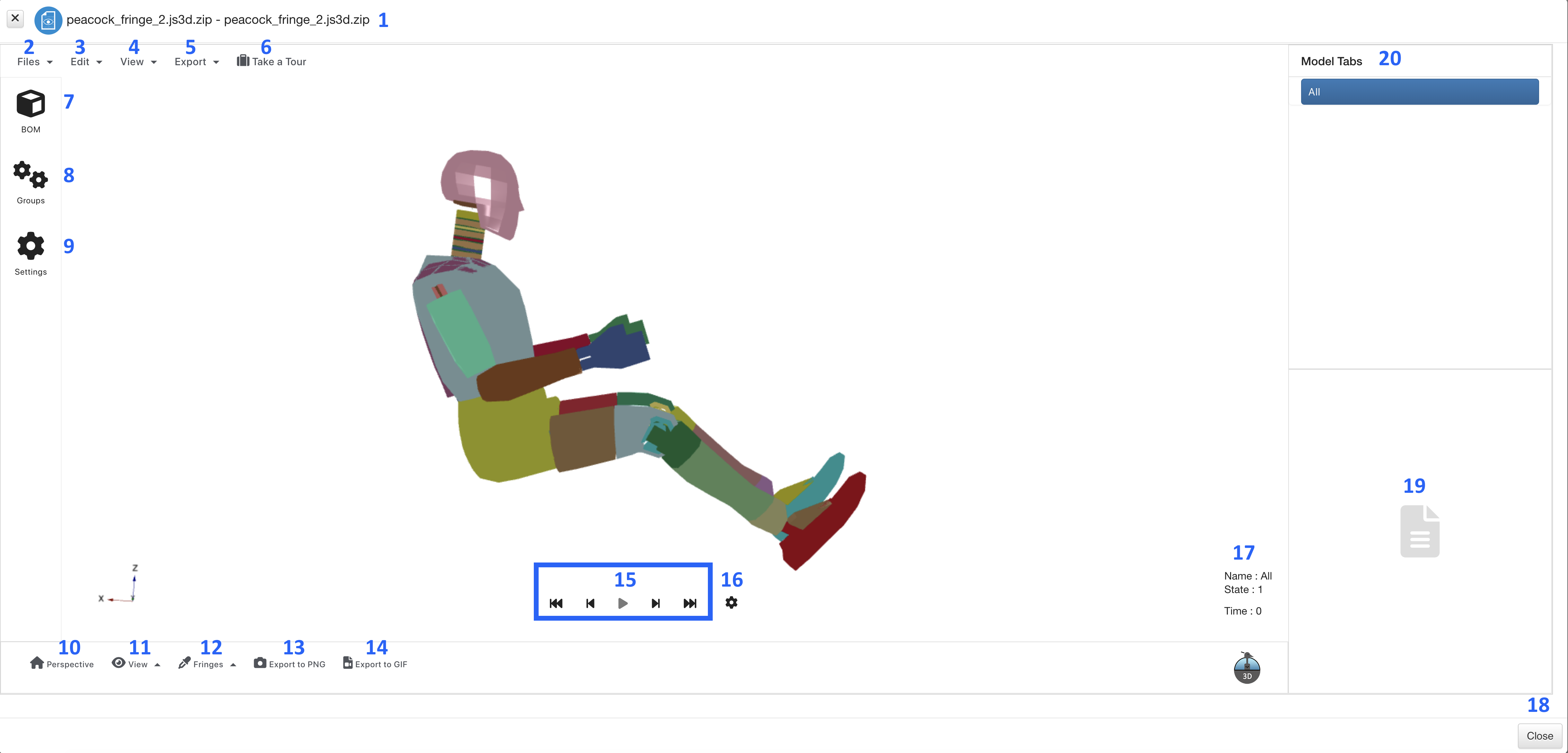
Figure 12: Peacock Interface
- Model file name
- Files: import more models
- Edit: turn fringes on/off
- View: change the perspective of the model
- Export: download the model as a GIF or PNG of current view
- Take a Tour: guided tour of Peacock basics
- BOM: view and edit Bill of Materials
- Groups: view, upload and edit assembly groups
- Setting: customize the experience such as changing the lighting or background color
- Perspective: takes us back to the Home view
- View: another way to change perspective
- Fringes: another way to turn fringes on/off
- Quick Export to PNG
- Quick Export to GIF
- Animation controls
- Settings for animation controls
- Animation information
- Close out of Peacock
- Information and controls will populate here when using certain features
- Model tabs: all uploaded model will be shown here for navigation
Perspective and Views
Click, hold and then move the mouse to explore different sides of the 3D model.
Use the View menus at the bottom or top of the window to see the model orthographically.
32.3. Features
In this section, we’ll go over some of Peacock’s useful features for exploring models.
Customization
Under the settings menu to the left, we can customize aspects of our model and experience in the 3D viewer.
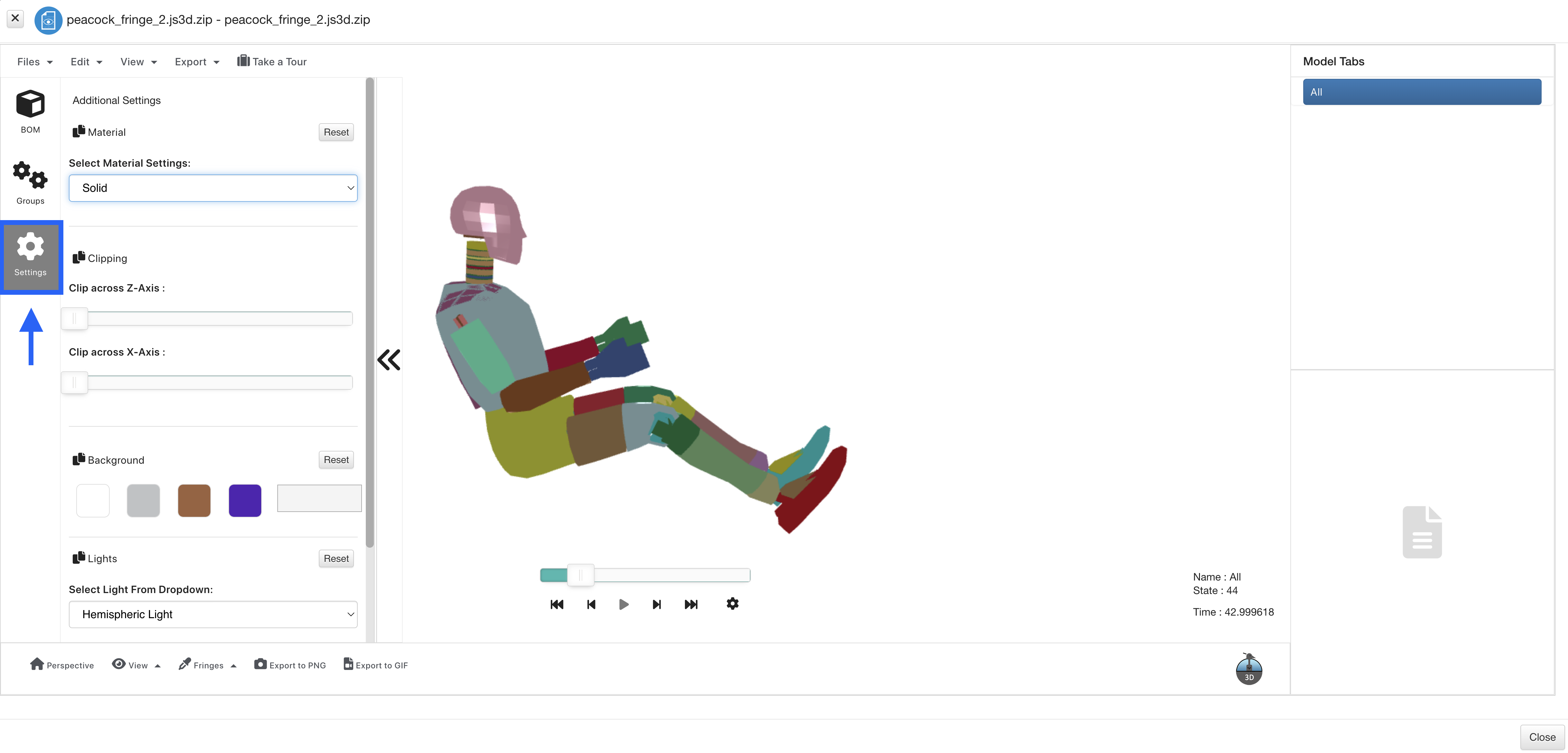
Figure 13: Peacock Interface
Edit the material type, clip the model, change the background color, choose different lighting and measure our model all under this menu.
Bill of Materials
Under the BOM (cube) menu, we can review all our model parts.
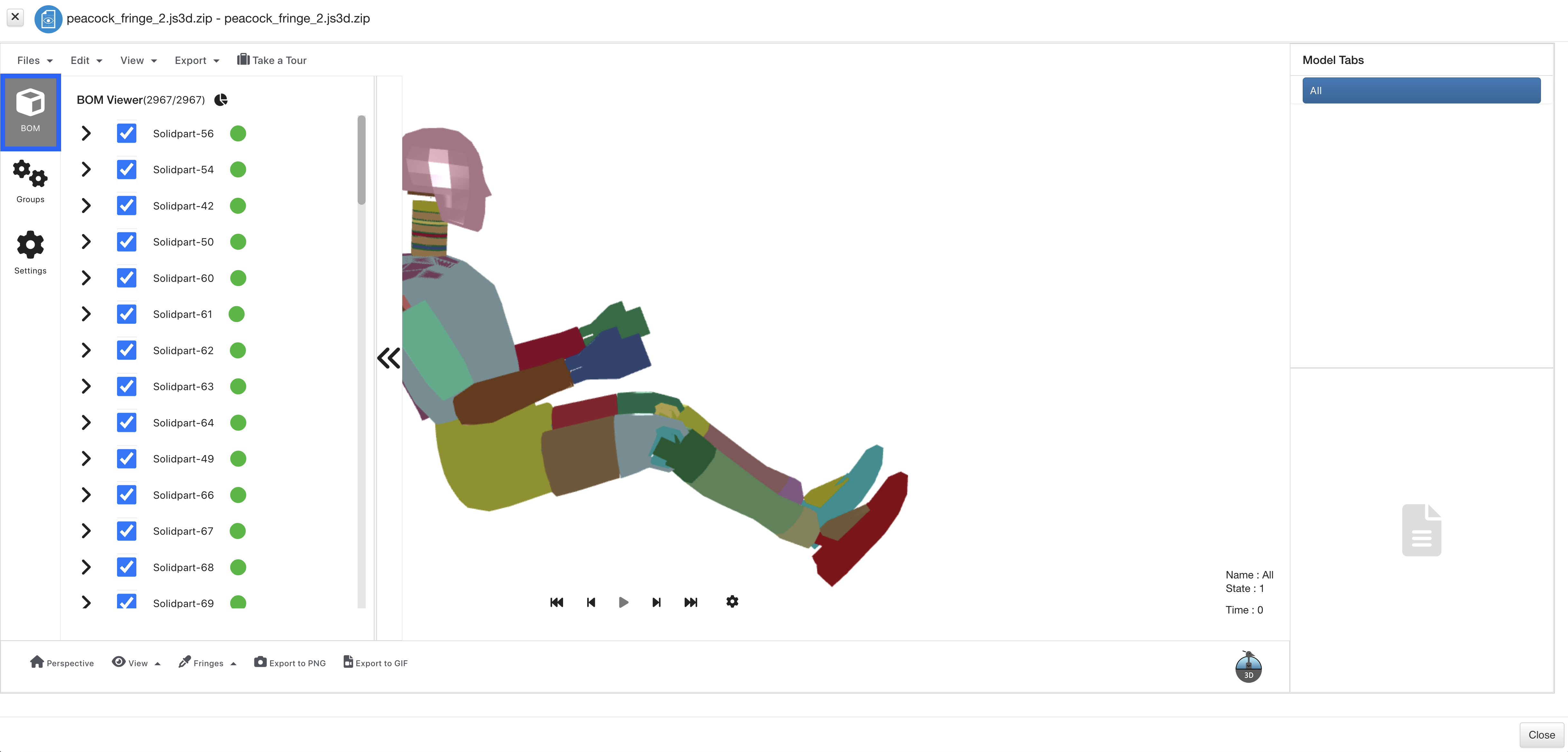
Figure 14: Bill of Material Menu
Click on the pivot caret to see information about a particular part and customize it.
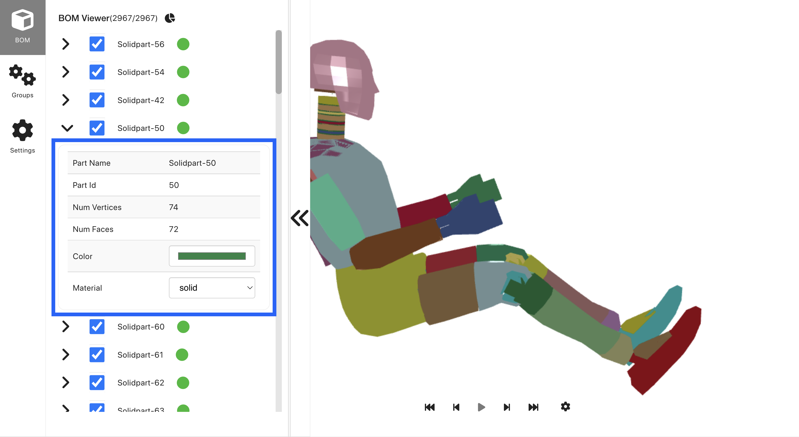
Figure 15: Bill of Material Part
We can update the part color as well as change the material type from solid to wireframe.
Uncheck parts to hide them from the model. Recheck to add them back or use the right side panel to restore them individually or restore them all.
Right-Click Options
Right-click on a model part to see the right-click options.
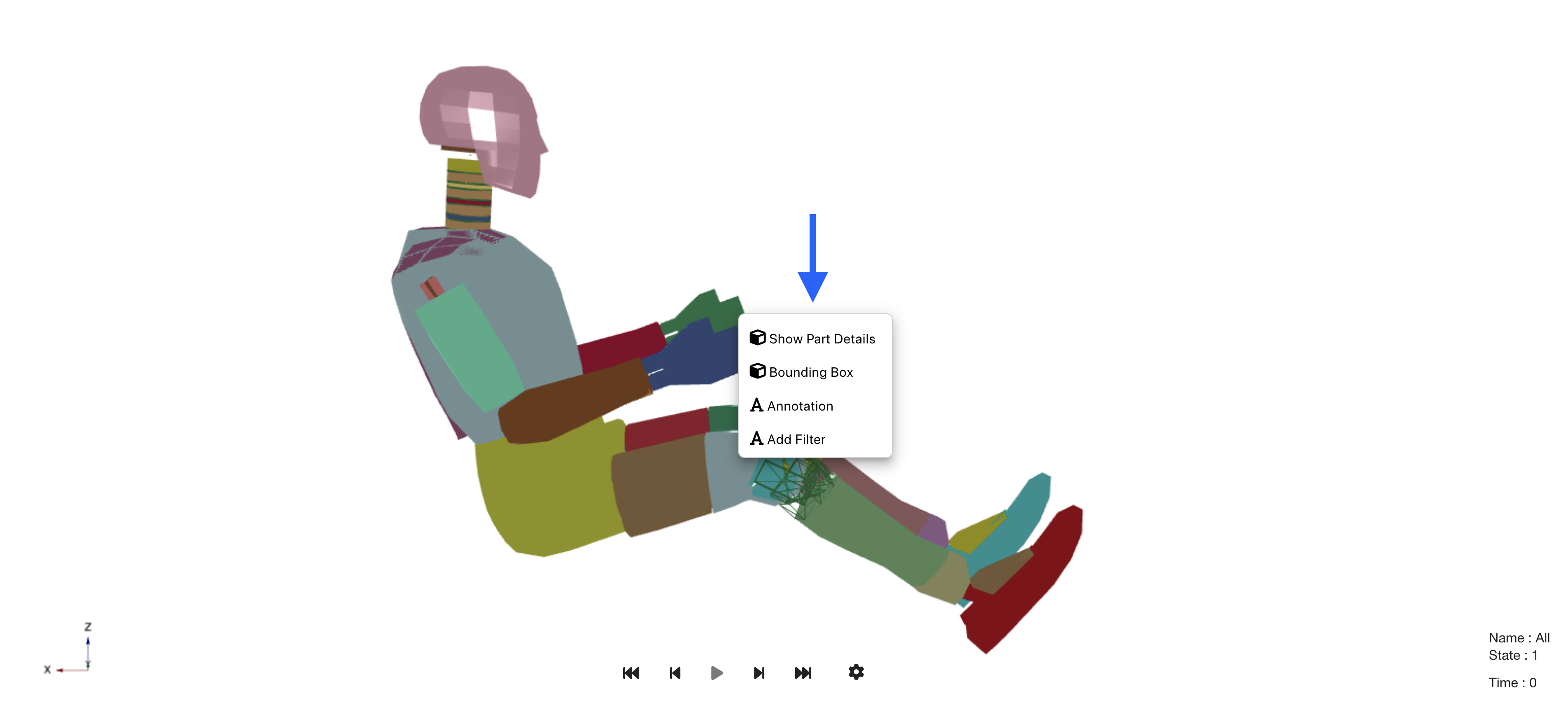
Figure 16: Right-Click Menu
Show Part Details
Show Part Details gives use the same information and customization abilities as the BOM menu for individual parts.
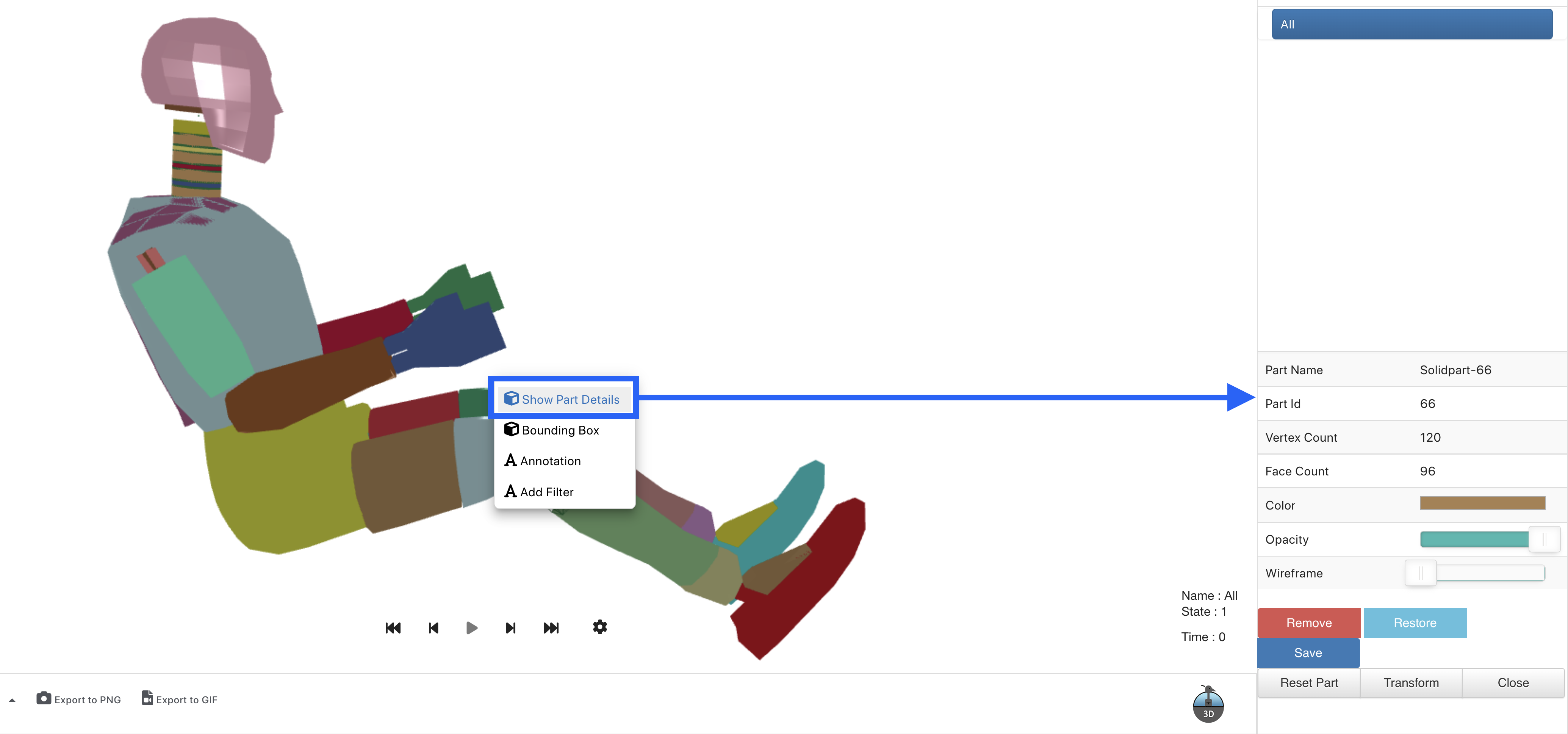
Figure 17: Show Part Details
We change the color and opacity, switch to wireframes, remove and even transform the model part. Make sure to click on Save to apply the changes. We can also use the Reset Part option to revert it back to its original settings.
Bounding Box
Bounding Box allows us to select groups of the model by using a selection box. We can choose the keep or remove selected elements in the right side panel.
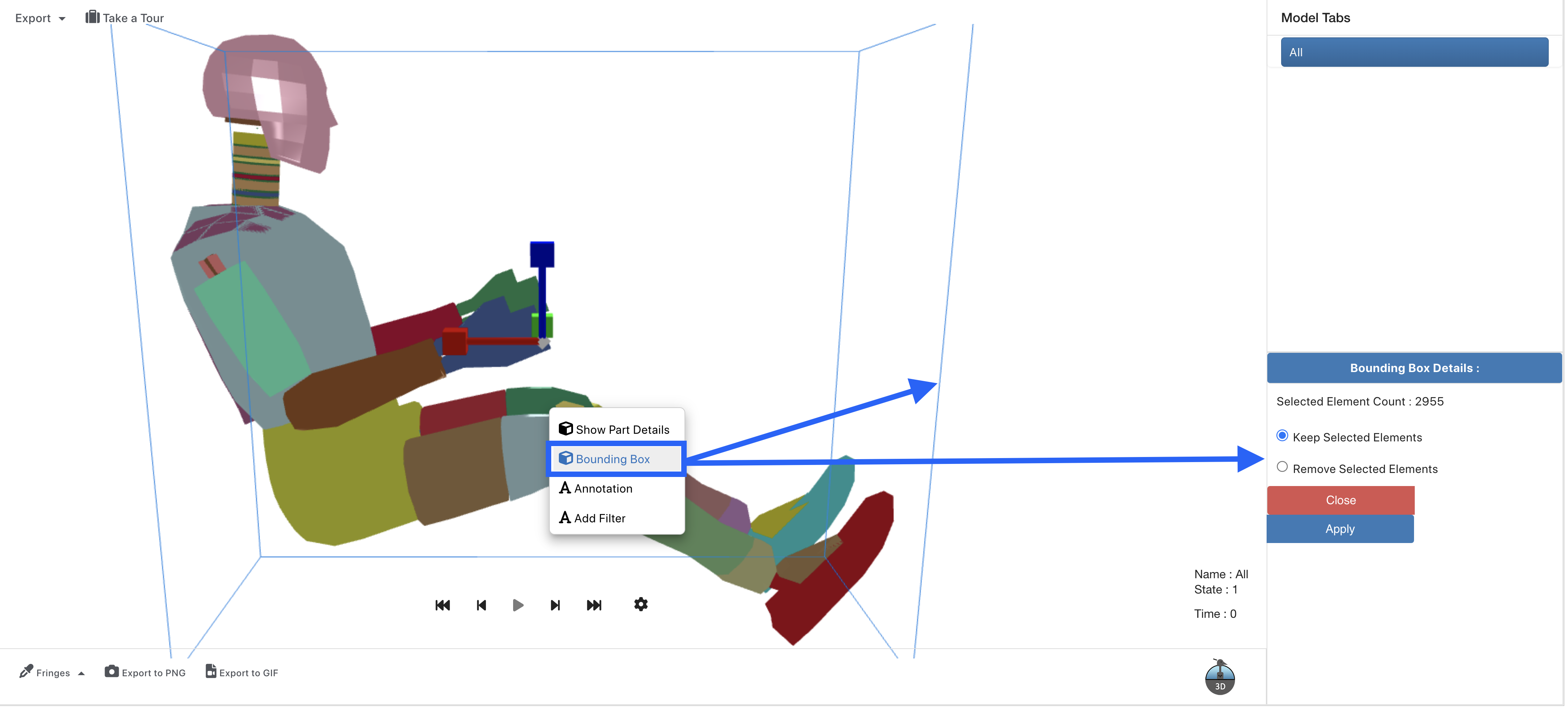
Figure 18: Bounding Box
Use the axis lines to resize and move the bounding box. Once we have our desired parts selected, we can choose to keep or remove the select parts and faces. Keeping excludes the rest while removing excludes the selected. If we choose to remove the selection as shown in the following video, we can create a section cut of our model.
In the right side panel, we’ll notice that the removed aspects of the model are listed as faces since we may have not selected full model parts.
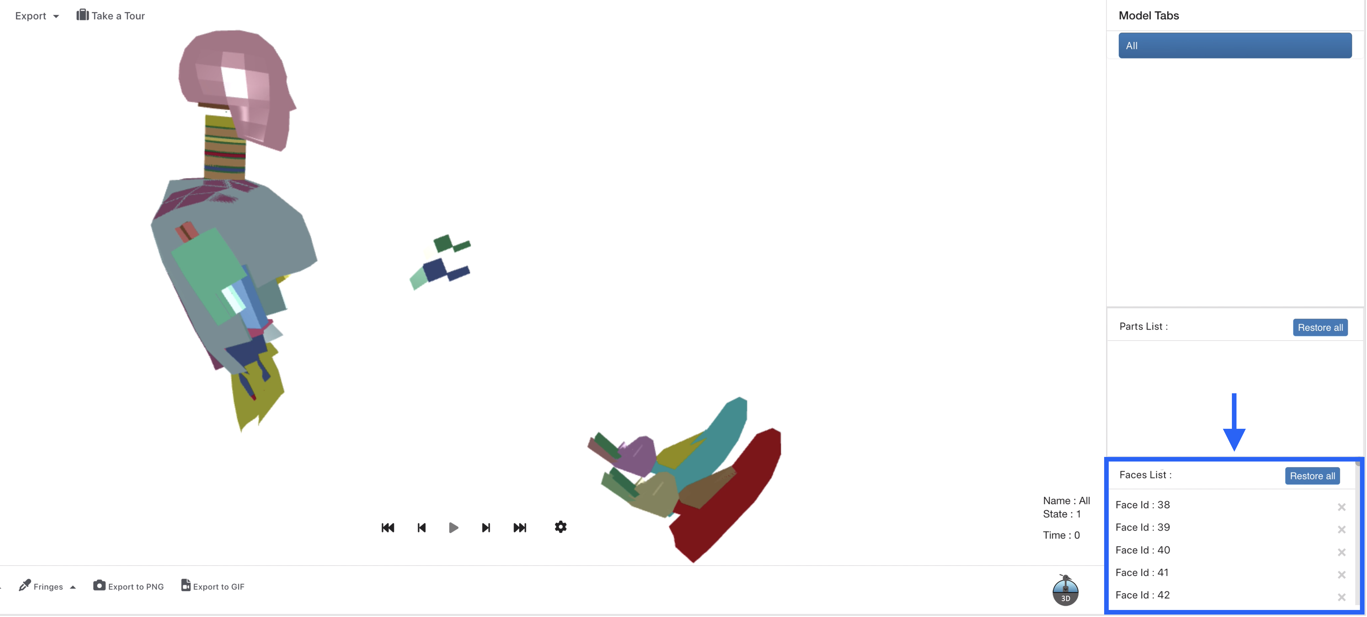
Figure 19: Removed Faces
Just as with our parts, we can restore individual faces or restore all.
Fringes
Peacock has fringe options for nodal and time-histories from LS-DYNA such as plastic-strain, von-mises-stress and triaxiality.
When extracting a JS3D response, make sure to indicate which type under the fringe parameters.
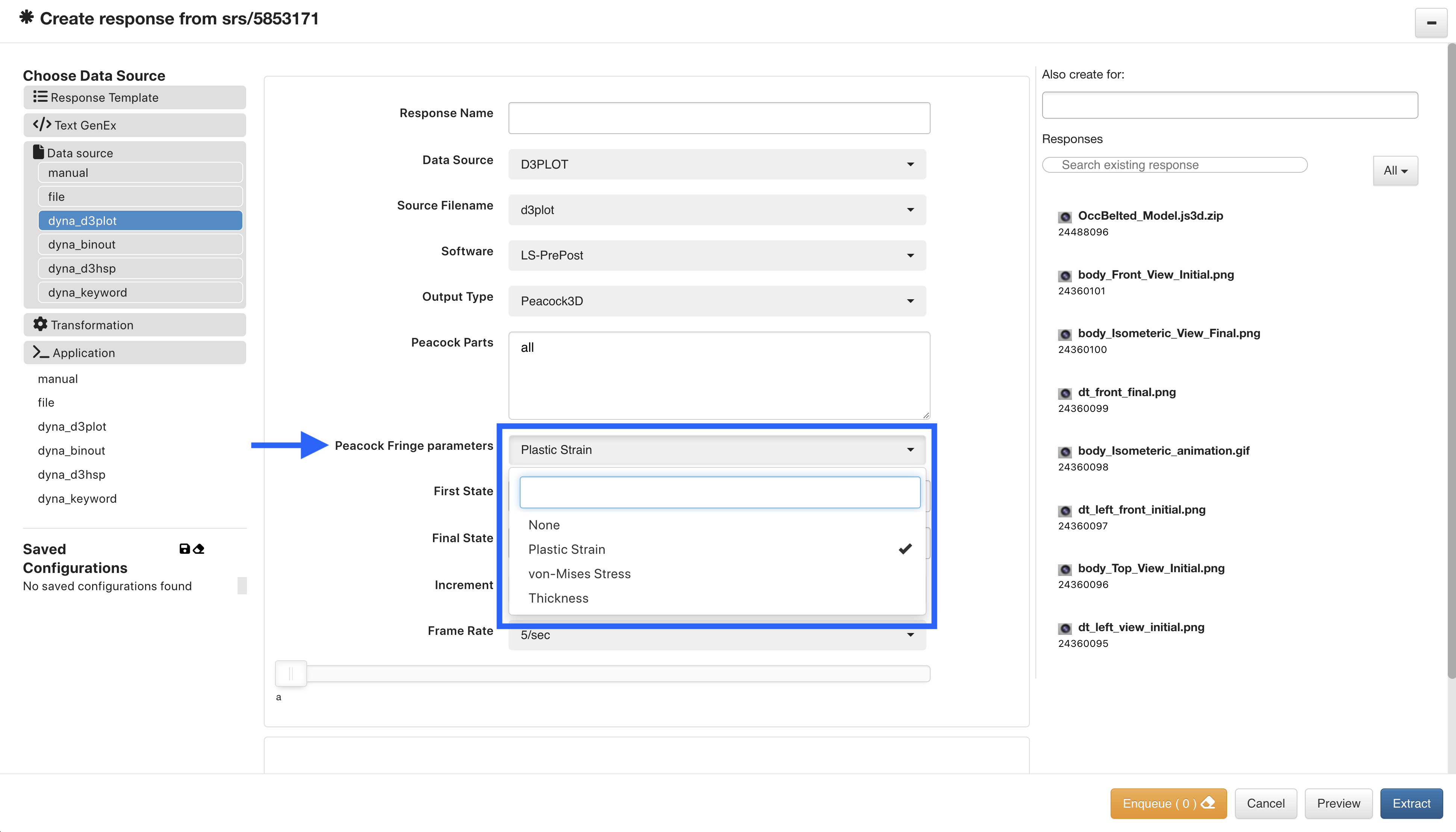
Figure 20: Fringe Parameters
Once we’re in Peacock, we can turn on fringes under the respective menu.
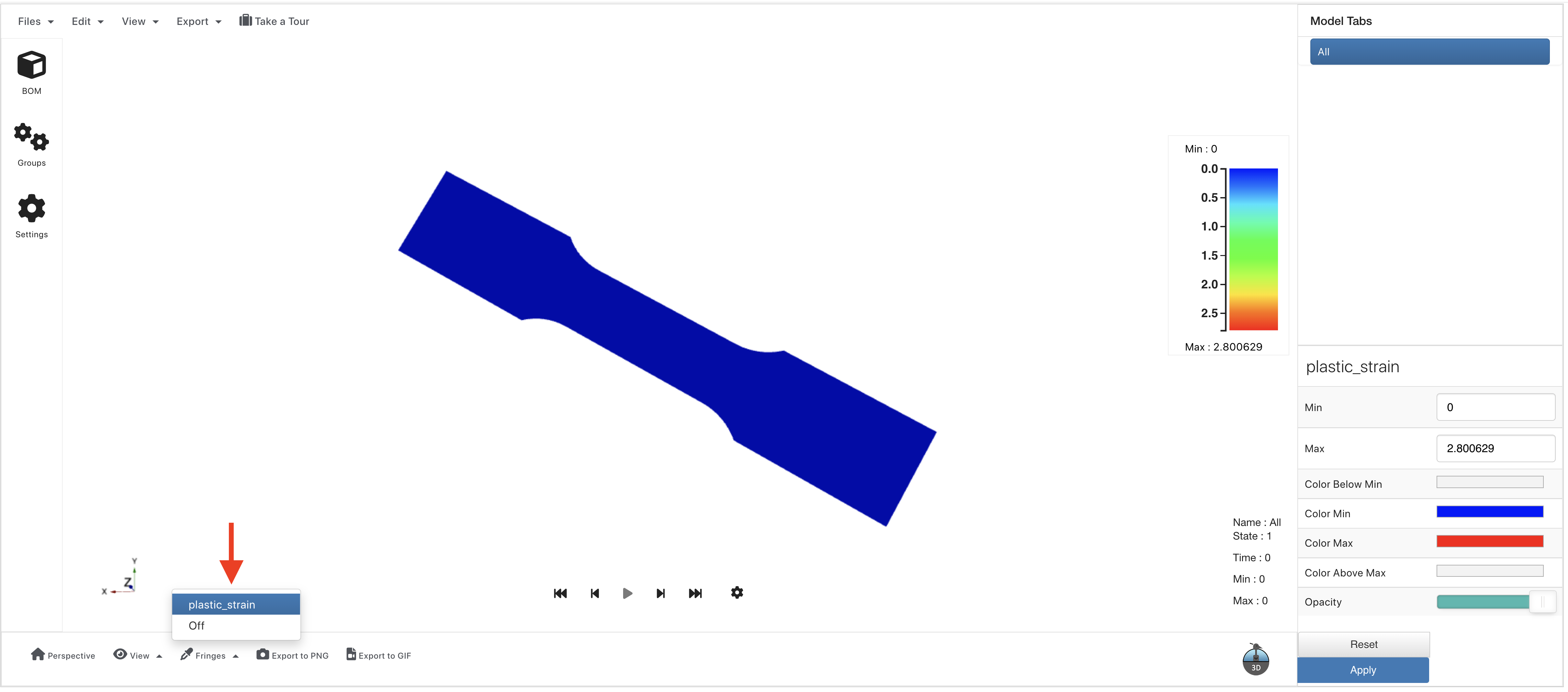
Figure 21: Turn On Fringes
We’ll see fringe spectrum (1) on the right side of our model canvas and our fringe settings on the right side panel.
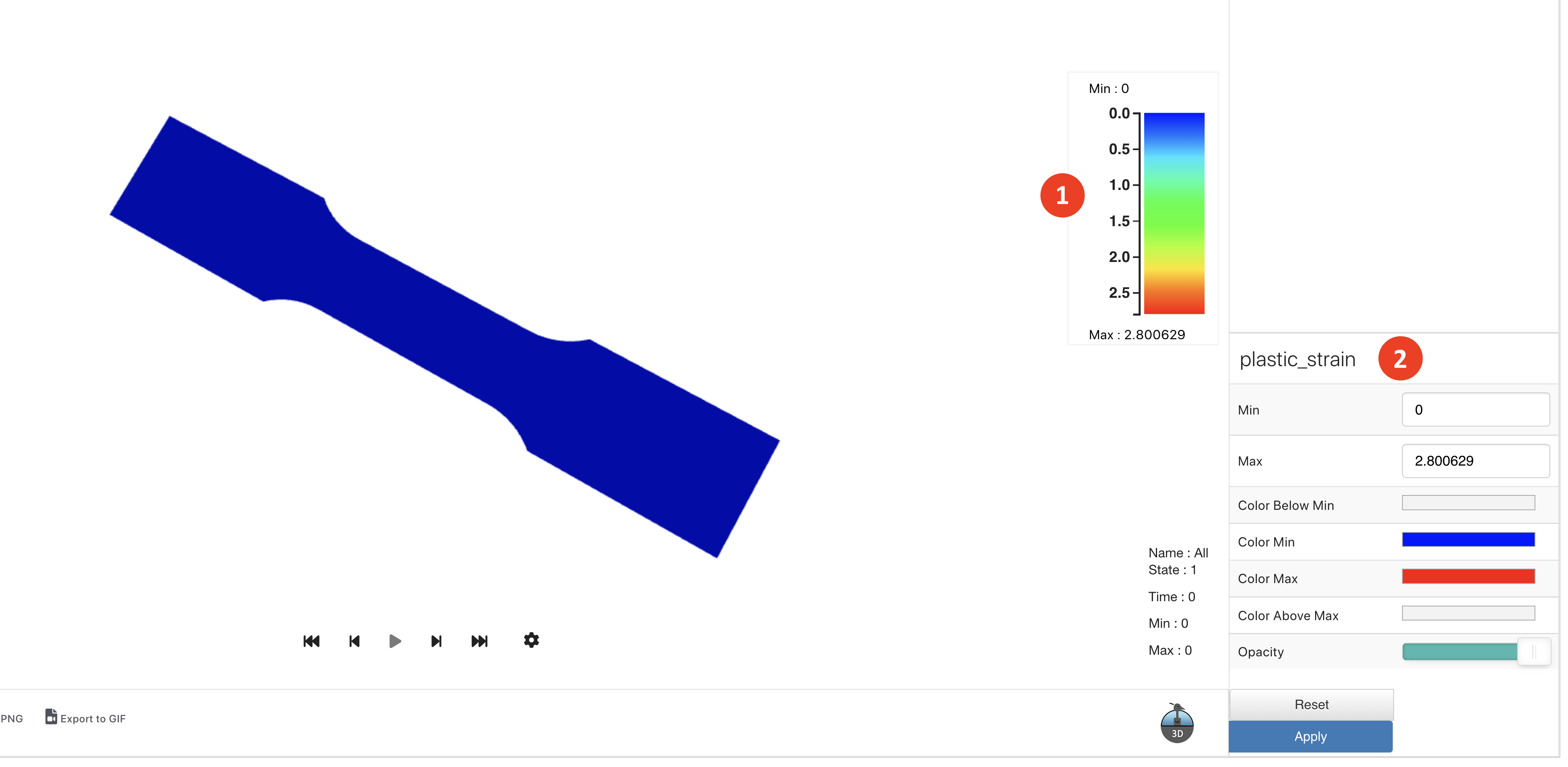
Figure 22: Fringe Spectrum and Settings
After we make any necessary updates, we can play our model to see changes in its fringe colors.
Assembly Groups
Under the Groups (cogs) menu, we can visualize and upload assemblies from LS-Prepost, Primer or Meta-Post.
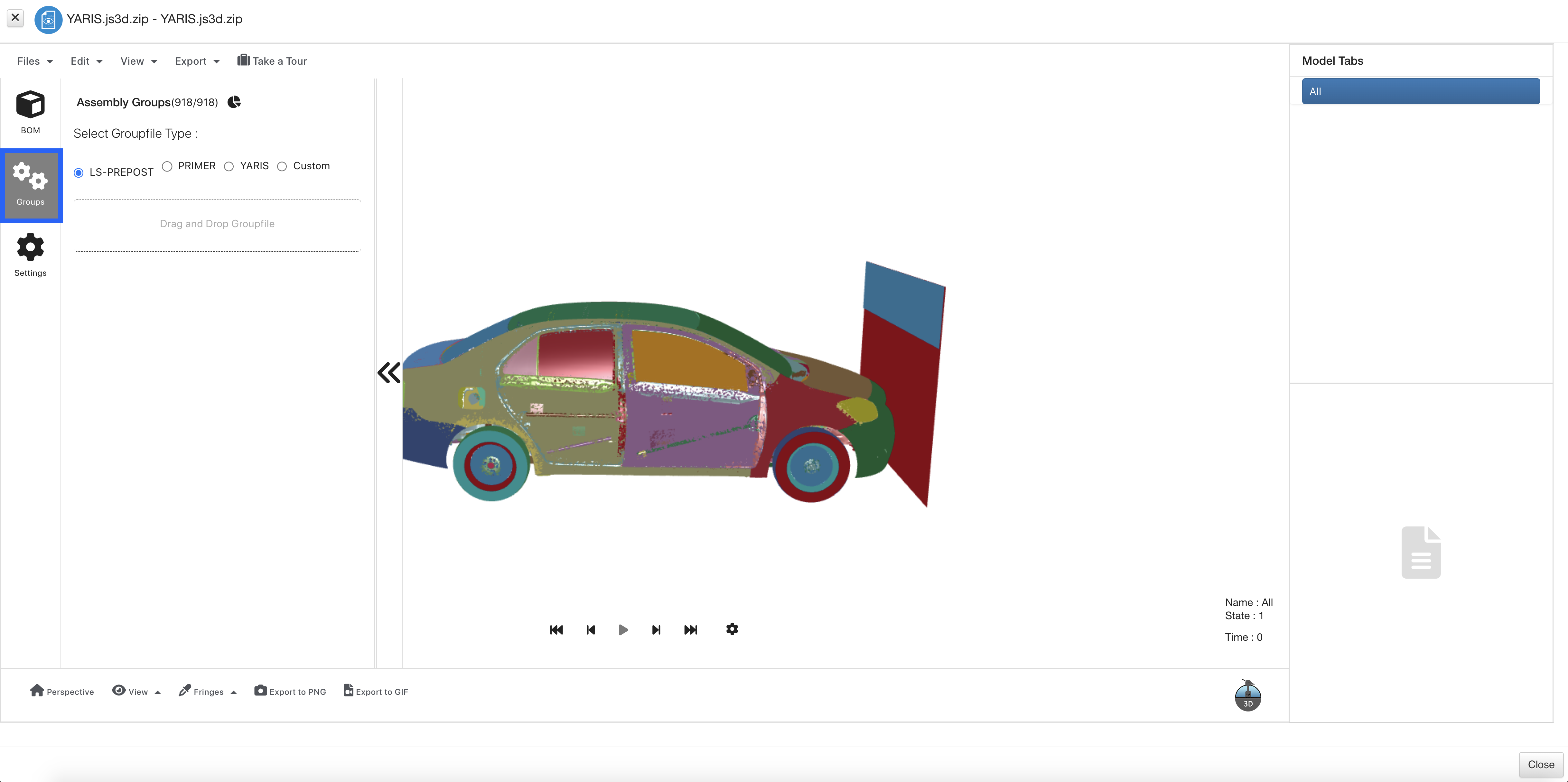
Figure 23: Assembly Groups
Choose the group file type (1), then drag-and-drop or click-to-upload (2) the group files.
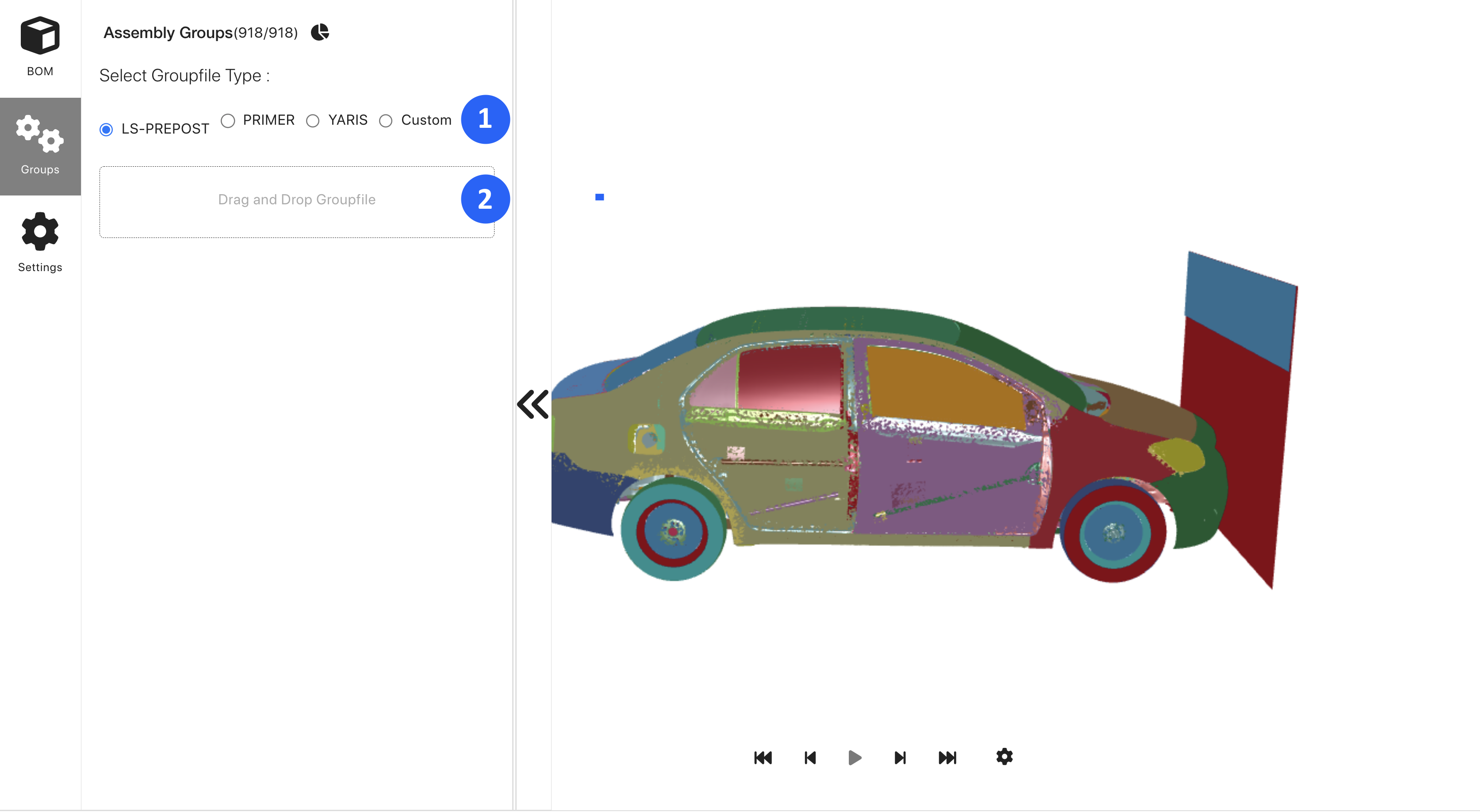
Figure 24: Add Group Files
Here is a video example:
Model Syncing
Aside from opening models directly from a simulation or physical test, we can also view and analyze these models in Simlytiks. We’ll do this by comparing responses of these simulations or physical tests. (Learn more in this section on comparing physical test responses.)
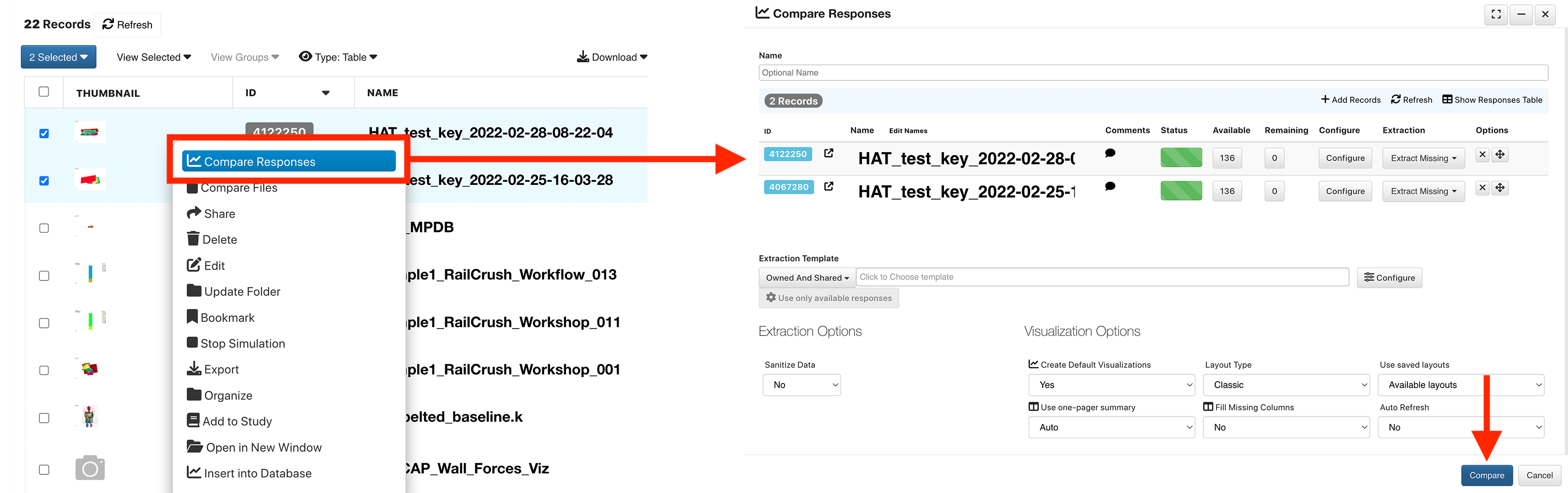
Figure 25: Compare Simulation Responses
Once in Simlytiks, we’ll create a new page (1). (Learn more on that here.) Then, we’ll drag-and-drop a model into the page section (2).
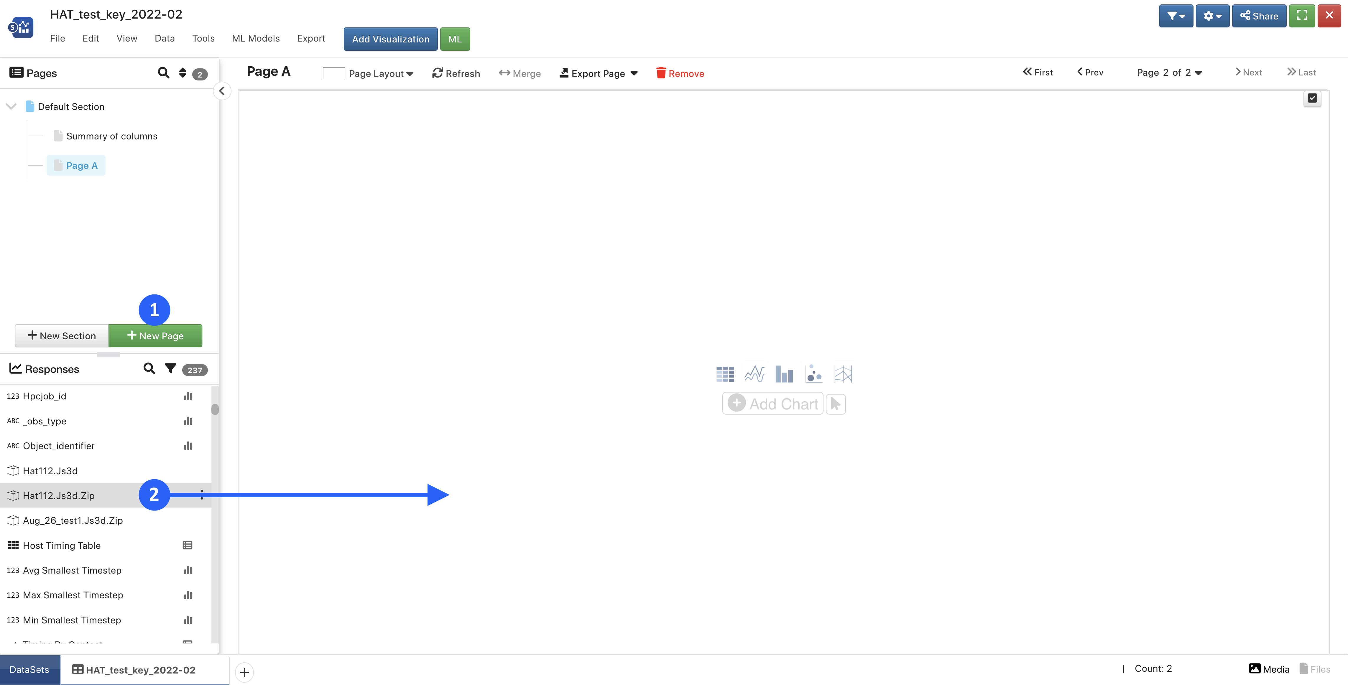
Figure 26: Add Models to Page Sections
We should see both models (one from each simulation we compared) appear on the page.
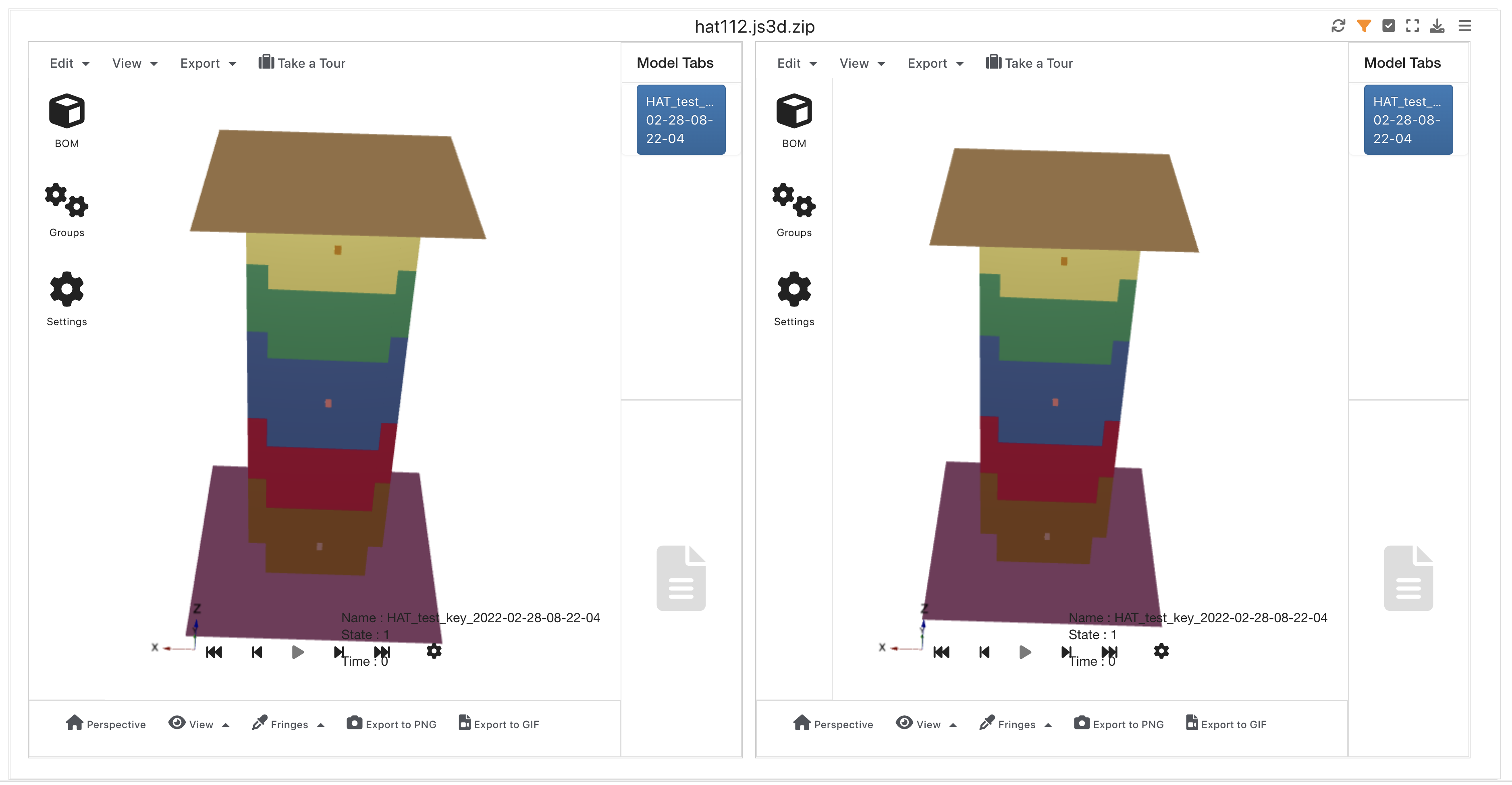
Figure 27: HAT Simulation Models
Now, we can perform any Peacock tools to one and see them reflected in the other.
This allows us to intricately compare the models in real time.
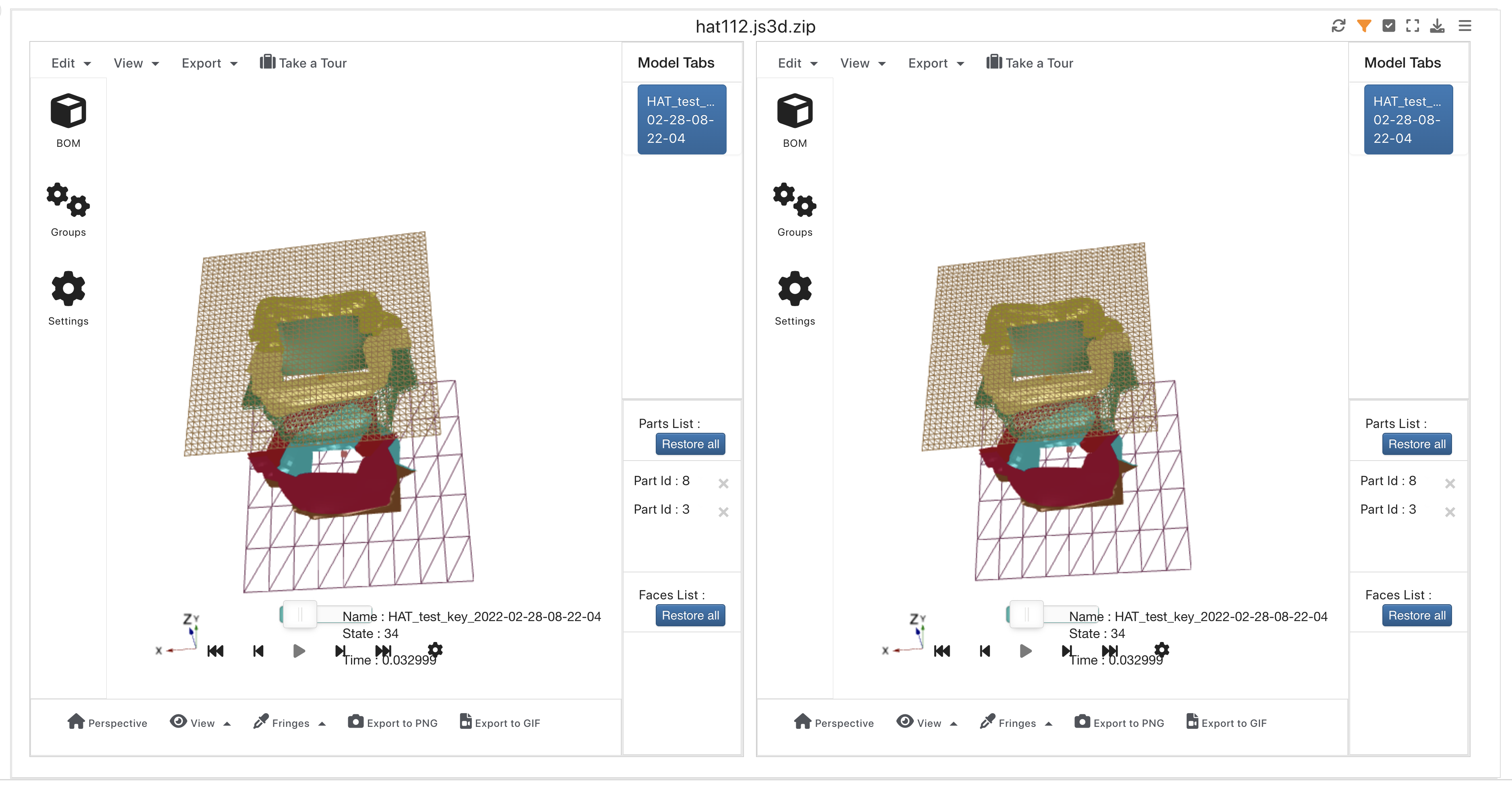
Figure 28: Synced Simulation Models
32.4. Sharing & Exporting
Let’s review how we can share and export our 3D model.
Sharing Options
The process for sharing our model will depend on if we extracted or uploaded it.
Share 3D Response
Our extracted 3D response can be shared, first, by locating it in the Response section of a simulation or physical test, then by clicking on the 3 dots in its top right corner. Under these options, we’ll choose Share.
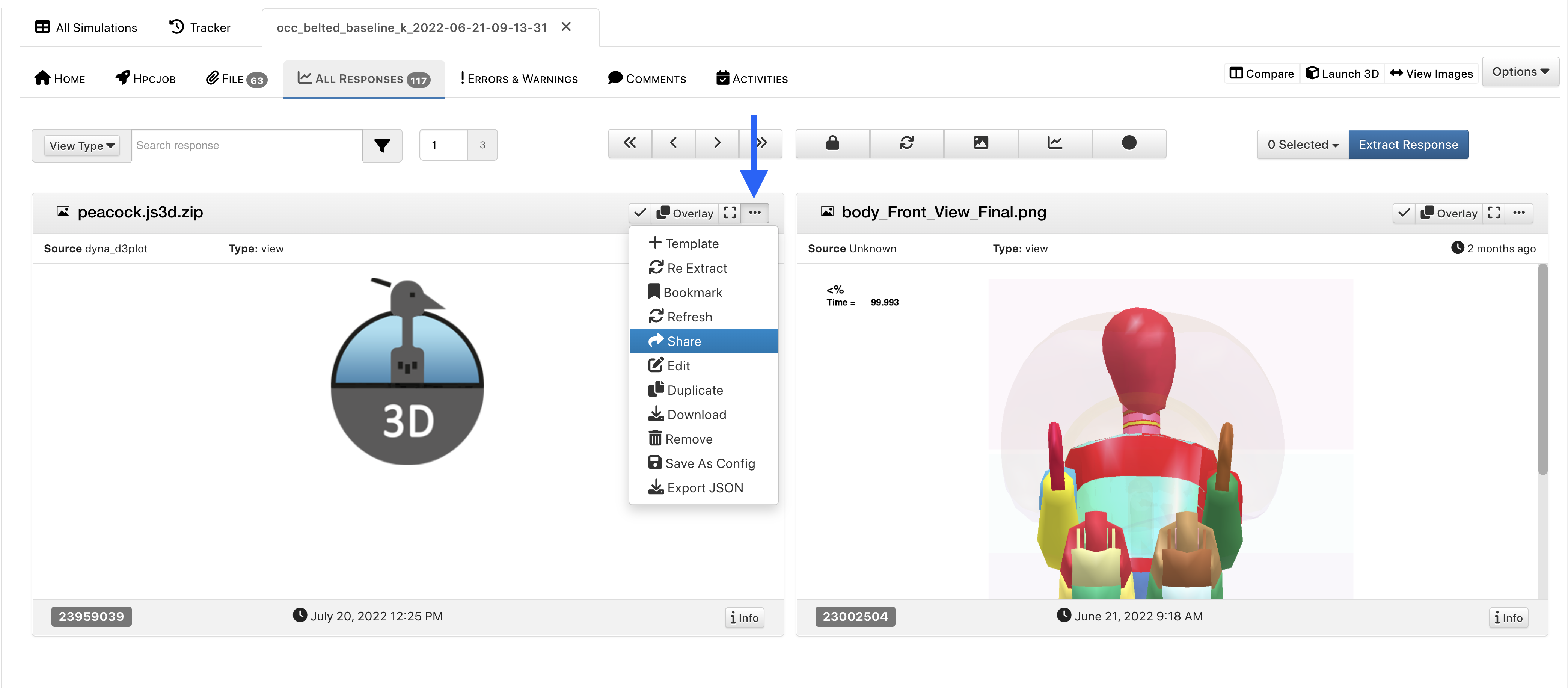
Figure 29: Share Extracted 3D Response
In the next window, we’ll indicate the type of share and then press OK.
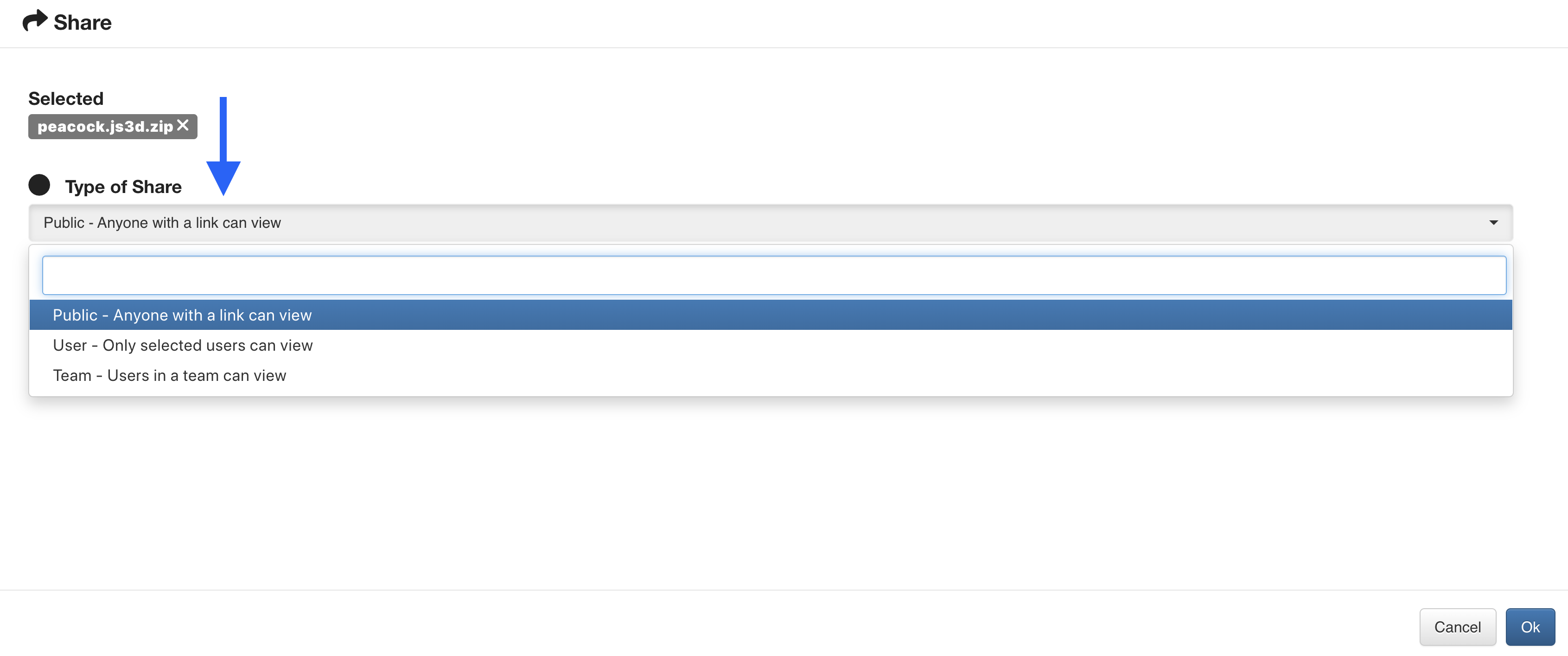
Figure 30: Type of Share
For this example, we’ve chosen a public share which has populated a link. This is the most common option as anyone with the link can view the model even if they do not have a d3VIEW account.
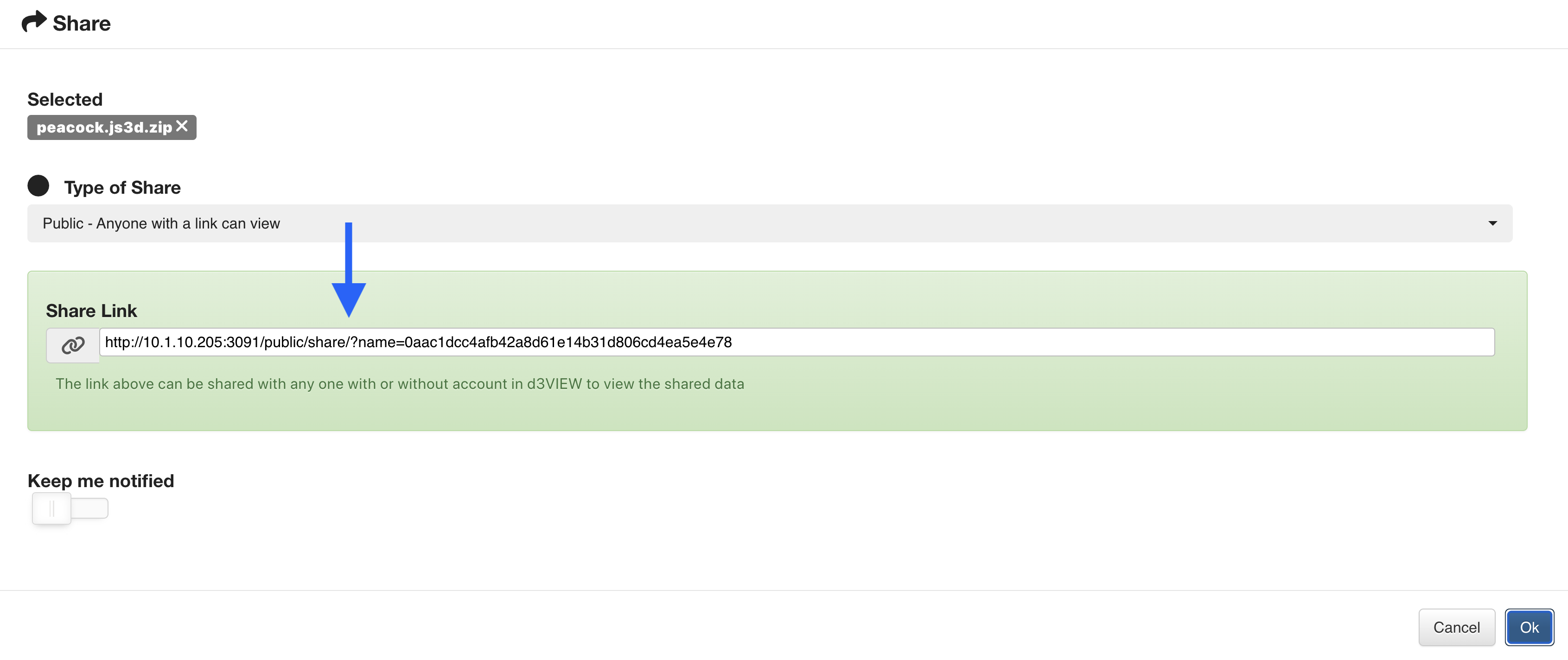
Figure 31: Public Share Link
Share 3D File
For uploaded model files, locate the model under the Files tab of a simulation or physical test, click the 3 dots and choose Share.
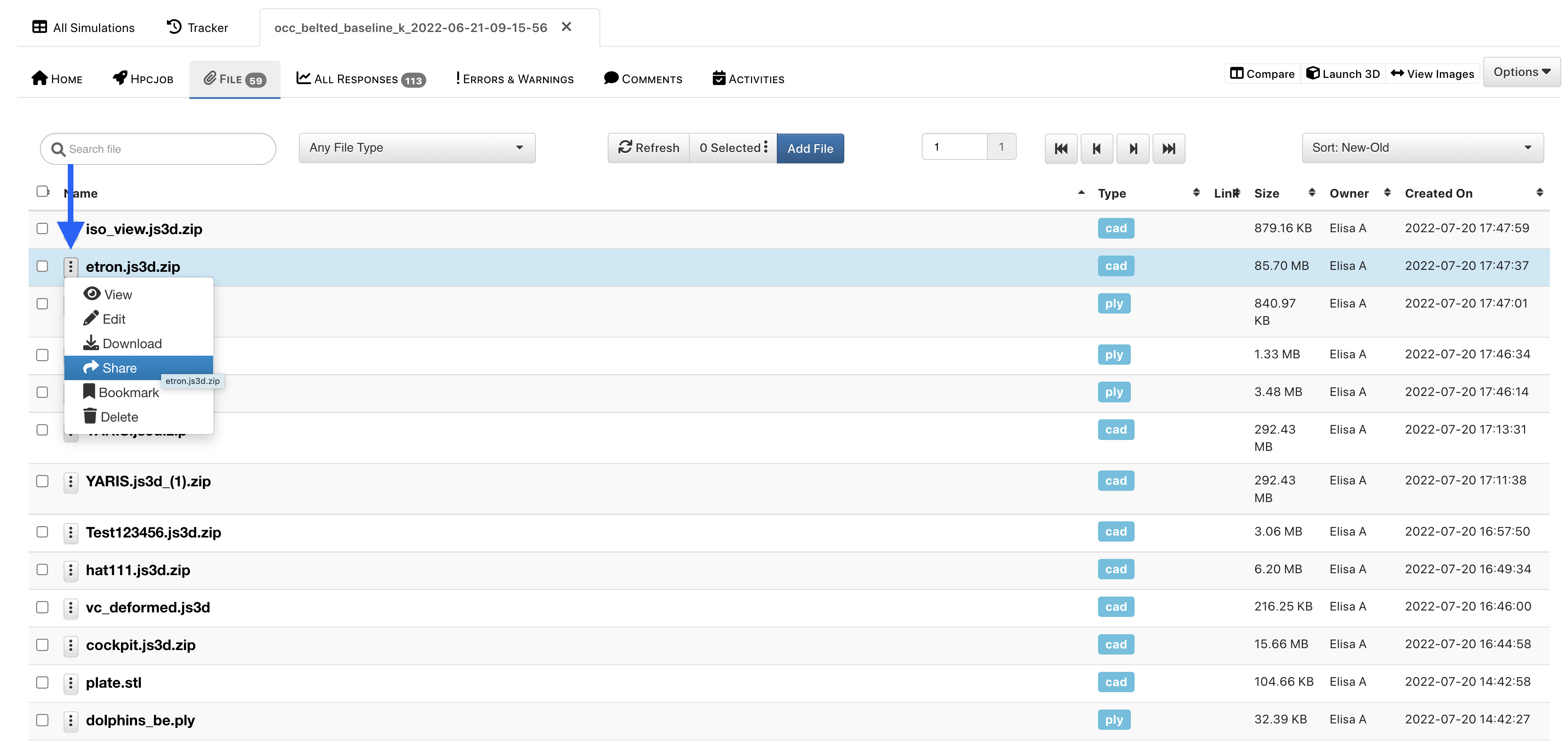
Figure 32: Share Uploaded 3D File
Choose which user to share the file with, then whether they can just read or read and write the file before pressing OK.
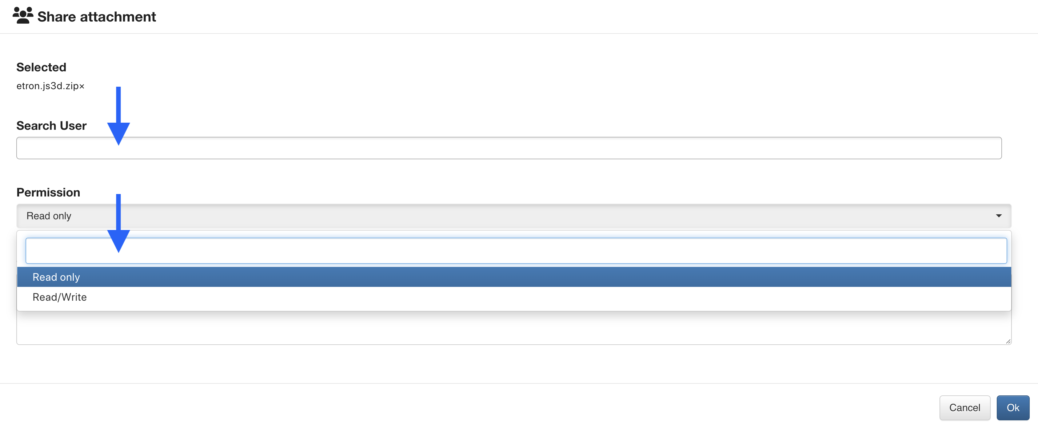
Figure 33: Choose User and Permission
Exporting Options
We can export our model via a PNG or a GIF. The PNG will be a still of the current view, while the GIF will be the full animation. Find these export options under the Export Menu at the top or as quick buttons at the bottom.
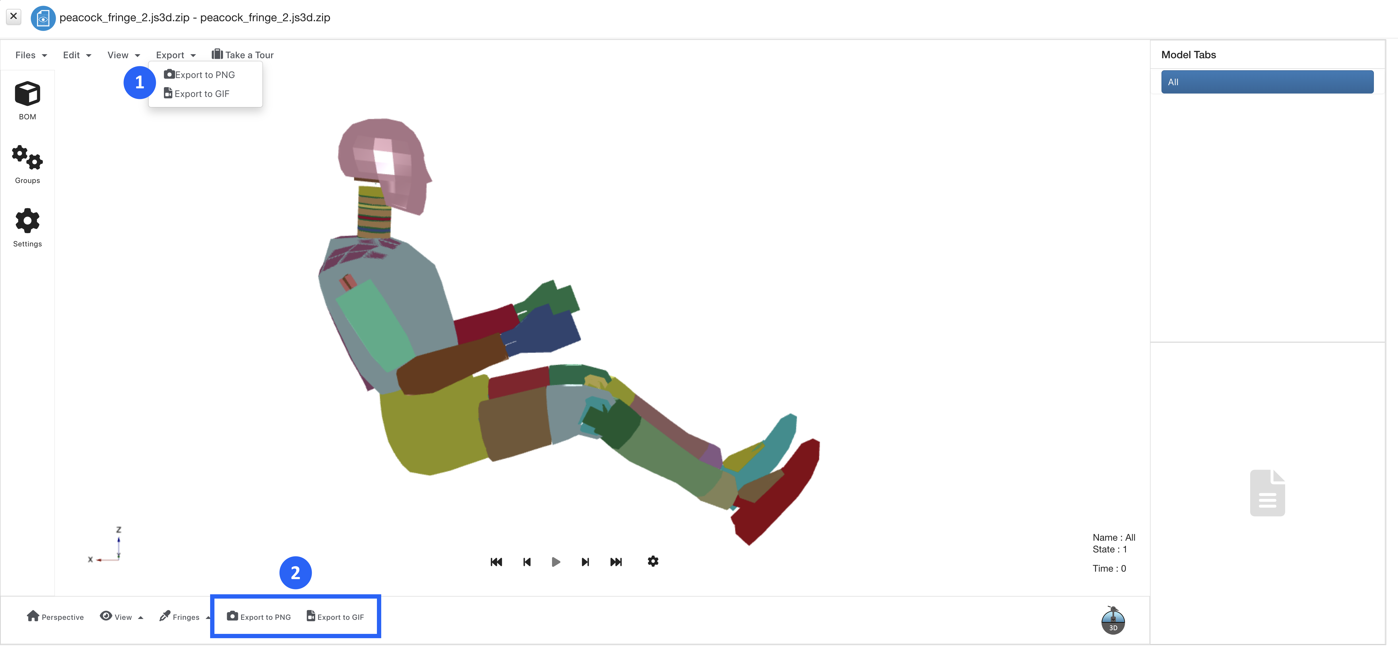
Figure 34: Export 3D Model
Download nodal co ordinates
Peacock modal has new Context menu option to download nodal coordinates as CSV.
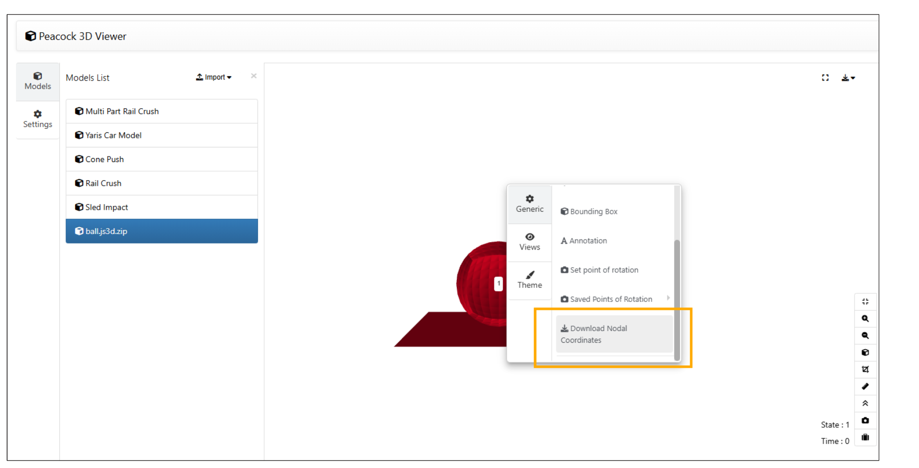
Download nodal co ordinates