18. BMS Publishing Guide

18.1. About This Guide

This guide provides an introduction on how to publish test-data from Battery Management Systems (BMS) from different labs such as CarTech or in-house systems to d3VIEW, a data-to-decision software that helps in scientific data-visualization.

18.2. Who Should Read This Guide

Engineers interested in publishing test-data from Battery Management Systems (BMS) to d3VIEW can use this guide.

18.3. What You Should Already Know

This guide doesn’t include how to install and setup the publisher (lucy). In order to install lucy, the correct version and environment need to be installed and configured.

This guide is written with the intention that engineers without any specific background can publish some tests to d3VIEW with lucy. However, certain familiarity with the following topics will greatly help with understanding

1. Basic computer skills
2. d3VIEW platform
3. d3VIEW data flow
4. linux commands
5. bash script
6. programming experience

18.4. Introduction

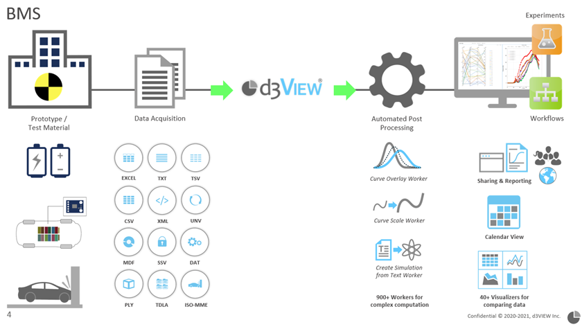
Battery Management Systems (BMS) provide a very useful data that allows to measure performance of batteries and aid in improving the battery performance. Several challenges exist while handling BMS data such as processing large time-history files, variety of different formats, viewing large data and performing analytics on them.

d3VIEW is a data-to-decision platform (www.d3view.com) that allows any Engineer, with little or no experience in programming, to import, process and store BMS data and provides advanced capabilities to view and analyze the data.

18.5. Getting Started

Overview of Data formats

Test data generated in the labs from experiments are collected and stored in various formats. There are mainly three major types of data in production and Table 1 provides a brief overview of these three types of data.

An overview of the three major types of data in production

Data Type	Pack Data	Cell Data	Others
Example	BMS.ssv other files	Filename.csv	Filename.csv
Source of Meta-data	WR file (not mandatory)	File name	Header section inside the data file
Data starts at Row	1	6	46
Column separator	Semi-colon (;)	Comma (,)	Comma (,)
Number of responses	700-1000	5	700-1000
Size	10-300 MB	~100MB	300MB-6GB

BMS Data

BMS data are stored in .SSV file with their meta data stored separately in a .WR file. An additional Completed.txt file is created to indicate that the test is complete and ready to get published. These files together are stored under a directory named after the test name. BMS data directories are grouped by the year the lab experiments are planned to be conducted.

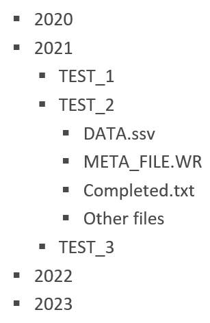
BMS data are grouped by year and their data files are stored in a directory named after the test name.

In the DATA.ssv file, the headers are defined as the first line while the data is defined in subsequent lines. Both the headers and the data are separated by the delimiter ‘;’. There are usually hundreds of signals for each BMS test and tens of thousands of points for each signal. Pack data may contains missing data where their values are left blank.

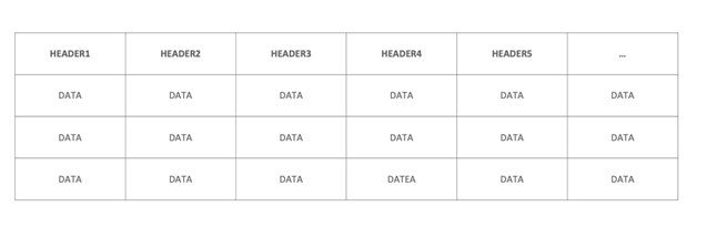
Illustration of pack data organization. Pack data are grouped by year and their data files are stored in a directory named after the test name.

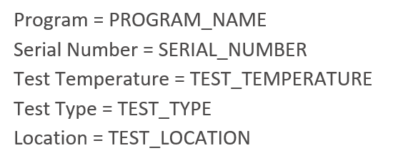
Illustration of WR (work order) file. Each line represents a meta-data which is used by d3VIEW to associate with the test that corresponds to this file. For example, the ‘Temperature[degC]’ is used to associated with the tag which allows published tests to be search by attribute.

Others

Some data are stored in CSV files. At the start of each data file, there is a header section of that contains all the meta data. The test data starts from after the headers and follows a similar structure as the pack data test file, but with a comma ‘,’ for delimiter. They also share a similar number of signals as pack data for each test. These test data usually have considerably larger number of points so that the size can be up to 6GB.

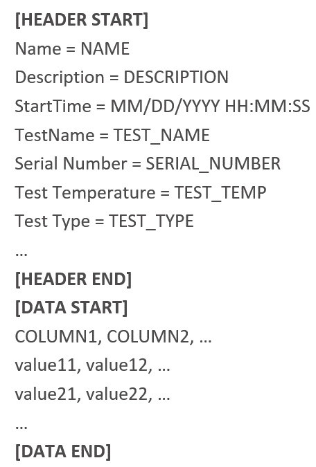
Illustration of test data with metadata as headers inside the CSV file.

Meta data “program name” is extracted from “Name”. One type of such “name” is in the format of “A_LC_B_SW_CDE”, where “LC” is the 2-letter abbreviation of the test location and “SW_CDE” is the software name. Together, “AB_SW_CDE” forms the “Program Name” to be used in the mapping procedure. Some of these test data stored in csv files are converted from the .MF4 file. We also support publishing the raw MF4 file without the csv version on the condition that the string “LC” appears in the MF4 file name.

Summary

In summary, the BMS data is stored in different data-formats as seen above and it is critical to support them by any data-visualization software. The publisher, provided as part of d3VIEW, supports these different data formats and provides a simple way to detect them and to publish them. If you have a data-format that does not match the ones listed above, you can contact your local support so d3VIEW’s publisher can provide readers for them.

Overview of publishing procedure

Experiments are performed in labs by engineers and test data are collected and stored in various formats. These data then will be shared with d3VIEW and get published to d3VIEW platform. Once test data is available on d3VIEW platform, they can be accessed, shared by engineers and a variety of visualization and analysis tools are available to users.

Publishing data flow on d3VIEW

There are two different ways to publish the test-data to d3VIEW.

In the first method, CLI-METHOD, we use Linux/Windows/Mac and use the Terminal to provide Command Line Interface (CLI) to call the publisher. The advantage of this method is it can be used directly in the terminal (CLI-METHOD-A), can be called programmatically inside BASH scripts (CLI-METHOD-B), and lastly, they can be called as part of scheduled tasks, such as CRONJOBs (CLI-METHOD-C), to watch a directory and import them as new test-data arrive.

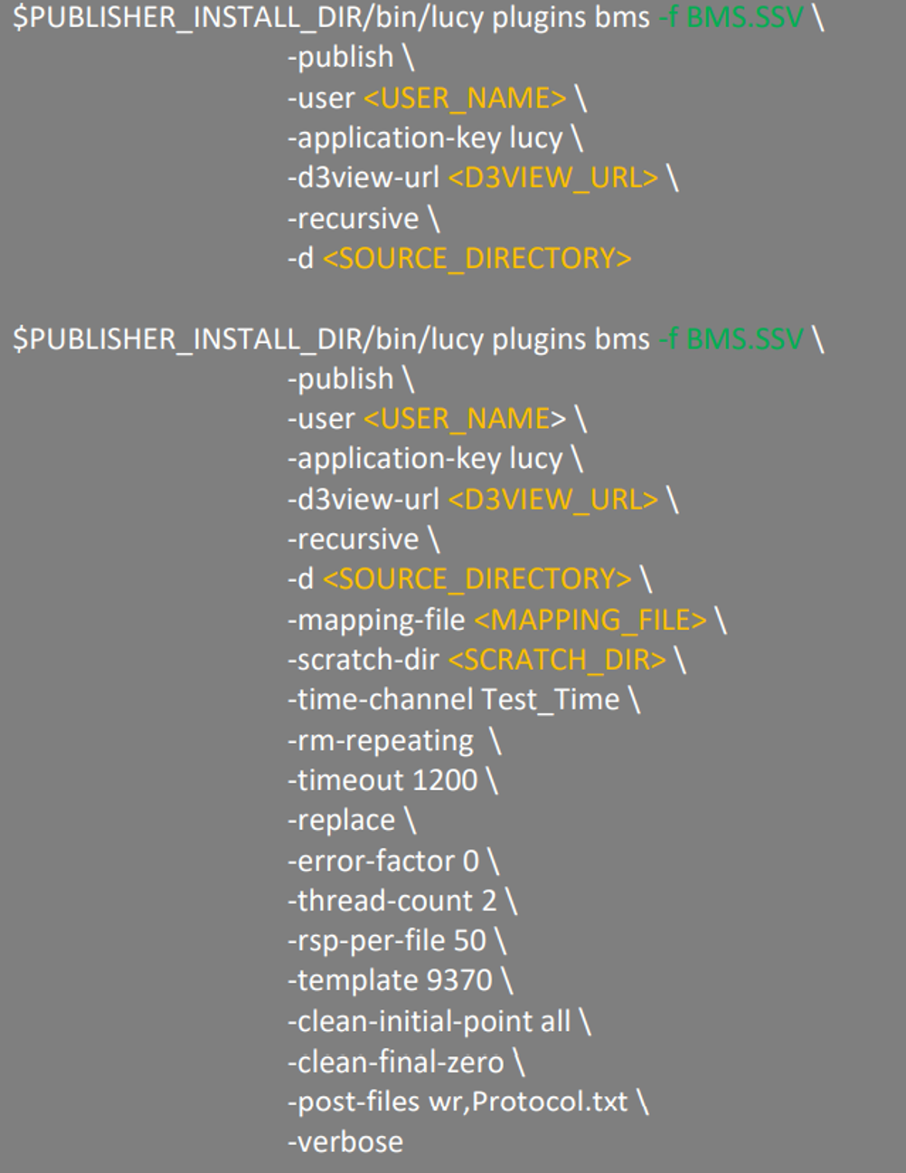
Two examples of the command format with different publishing options to be used for publishing using CLI-METHOD-A method.

We can also put the commands in a BASH script and provide instructions for the publisher to automatically identify test data to get published.

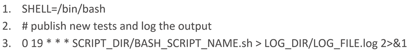
A sample CRONJOB set up in the CRONTAB file to be scheduled at 7pm every day and save the logging in the specified file.

Users can choose their preferred method to publish the test data. Here is what needed to publish in general:

1. A file or directory that contains test-data.
2. Publishing commands or a BASH script for CLI-METHOD method (provided by d3VIEW).
3. Python enabled Linux/Windows/or Mac with necessary modules (Please refer to the Lucy Administrators Manual).
4. Latest Lucy Binary (provided by d3VIEW).
5. A licensed version of d3VIEW to where the data can be published

Publishing command and options (CLI-METHOD-A)

CLI-METHOD method calls for the “bms” plugin from where the publisher (lucy) is installed to perform the publishing task in a manner controlled by the publishing options. The directory where the publisher is installed must first be specified in the publishing command for the CLI-METHOD-A method (Figure 9), followed by calling the “bms” plugin and publishing options. BMS, Element and EMEA test data are using “bms” plugin to get published while CarTech test data are published by using “cartech” plugin. Both plugins share most of the publishing options.

Publishing options are instructions for publisher to locate the data file to be published, how and where they will be published. Depending on the requirements for publishing, each publishing task can have its own set of options. In production, BMS, Element and EMEA test data use “bms” plugin for publishing because they share a lot of similarities in terms of how their data are stored and structured. Table below provides an overview of some mostly used options used in publishing with brief descriptions.

Publishing options	Descriptions
-publish	Publish to d3VIEW
-user	A valid user on d3VIEW
-f	File name or regex pattern to search for (e.g., BMS.ssv, *.ssv, *.csv)
-application-key	lucy
-d3view-url	d3VIEW site where test data will be published to
-d	Directory to search for data files
-mapping-file	A mapping file used for publishing
-scratch-dir	Directory for publishing related scratch work
-match-type	Determines which program’s mapping table to be used
-time-channel	Raw channel names to be used for time channel
-error-factor	If abs(y_prev – y_curr)<error-factor*(ymax-ymin), then y_curr is dropped
-rsp-per-file	Max number of responses to be included for each responses.json file (n responses per file)
-template	Template to be applied
-project-name	Project on d3VIEW where test data will be published to
-recursive	Recursively search for data files under specified directory
-clean-initial-point	all: removes first point of each signal outlier: removes first point of signals whose value is an outlier 123: a scalar. this removes the points from the response whose absolute values are greater than the specified value.
-clean-final-zero	Remove the last zero for each signal
-post-files	Post specified files to FILES section in the published tests (e.g., wr, Protocol.txt)
-prefix	Add prefix to the published test names
-force-replace	Remove existing tests with the same name and publish new a test
-verbose	Display output and loggings
-user-mapper	True or False. This intends to map single digit Cell Voltage/Temp signals to the same number of digits as that of the max number by filling zeros allow multiple source names in one cell separated by comma
-skip-lines	Followed by a non-negative integer. It will take every other nth line from the original data if the number is greater than 1. Otherwise, it publishes every row of the raw data.
-normalize	Normalize data before applying rdp simplification
-rdp	Apply The Ramer–Douglas–Peucker algorithm to simplify signal curves
-csv_meta_mapper_file	Provide a mapper file for csv to map header information to Programs, temperature etc. The format is name=value where name is what will be in csv and value can be Description,Temperature[degC],Program,Test Name,Location,Serial #,Tested On

Publishing with a script (CLI-METHOD-B)

In CLI-METHOD-A method, we need to manually provide all the details explicitly every time we submit the command in Terminal. It has its advantage that we know exactly what have been passed to the arguments for each option. On the other hand, sometimes this can be quite cumbersome for the same reason. It requires considerable amount of efforts to make sure every detail provided is accurate. By contrast, CLI-METHOD-B method embeds the command into a BASH script and thus it provides the flexibility to automate at least part of the argument specification process. For example, instead of manually updating the path and the name of the test file, we can ask the publisher to search the certain directories by itself every time we run the script.

In order to automate the process of specifying all the arguments for publishing options, we need to specify the parameters to be used for gathering such information. Some commonly used parameters we need to set up are listed in the table below with descriptions about their purposes

Parameters	Descriptions
years	BMS data are grouped by year. Year must be specified so that we know which sub directory (under the ./data directory) to look for test data files.
from_dir_base	Directory for the data folder that includes the “year folders” (e.g., sub-directory named after year to store BMS data of different years)
to_dir_base	Data will be copied to this directory for publishing
debug	If we want to publish or just debugging
days	Tests older than these many days will not be published
pattern	We are looking for ssv files
lucy_install	Directory where lucy is intalled
bms_import_dir_base	Directory where data will be published
scratch_dir	Directory for lucy to do scratch work during the publishing process
bms_mapping_file	Path of the mapping file that will be used for publishing
bms_database_file	Path of the hevWrInfo.tsv file that will be used for publishing
d3view_url	Which d3VIEW app site the data are to be published.

At first, this may be intimidating that not only we need to specify the options but also take care of all these new parameters. However, right after it is set up (this is usually provided by d3VIEW), it will be so much more convenient when, for example, we want to publish the new test data from the same directory every day. We only need to run the script and the script will identify new test data, using the rule we set up by “days”, and publish them without manually changing anything.

Pre-requisites for Publishing BMS tests

Before publishing any test, the publisher needs to know if a test is ready to get published. There are three major files to check before publishing.

• Completed.txt

  • It is created when a test is completed, and its data are received. If it is missing, the test will not be published.

• DATA.ssv

  • It is the data file. If it is missing, the test will not be published.

• WR

  • It contains meta-data. If it is missing, the test will get published, but the meta-data will be empty or set to be default.

A BMS sub test is a test related to its parent test therefore it shares the same test name with the parent test but with an underscore followed by a number starting from 1 to indicate it is a sub test (e.g., TEST_NAME_1 is a sub test of test TEST_NAME). A sub test is stored separately in its own data directory and thus it is not different from other tests in terms of data organization and publishing except that it does not require to have a .WR file nor a Completed.txt file as long as its parent test does. This only applies to pack data since other test data are all stored in a single CSV file and they don’t have sub tests.

After we have configured the test, we can run the script. To run the script, we use either one of the following commands

sh SCRIPT_NAME.sh

or

./SCRIPT_NAME.sh

Scheduling CRONJOBs using CRONTAB (CLI-METHOD-C)

A CRONJOB is a command scheduled to be executed periodically at the specified time. With the flexibility brought by the CLI-METHOD-B method (publishing with a script), we can create a schedule of CRONJOBs that publishes test data periodically as they come in. In order to create a CRONJOB, we need to configurate the CONRTAB file that schedules it.

We can use the following command in the Terminal to check the existing CRONJOBs scheduled in the CRONTAB file.

crontab -l

With the “-l” flag, it prints out the content of the CRONTAB file and we can’t make any edition. If we want to edit the CRONTAB file to make changes, we can use the following command.

crontab -e

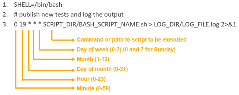
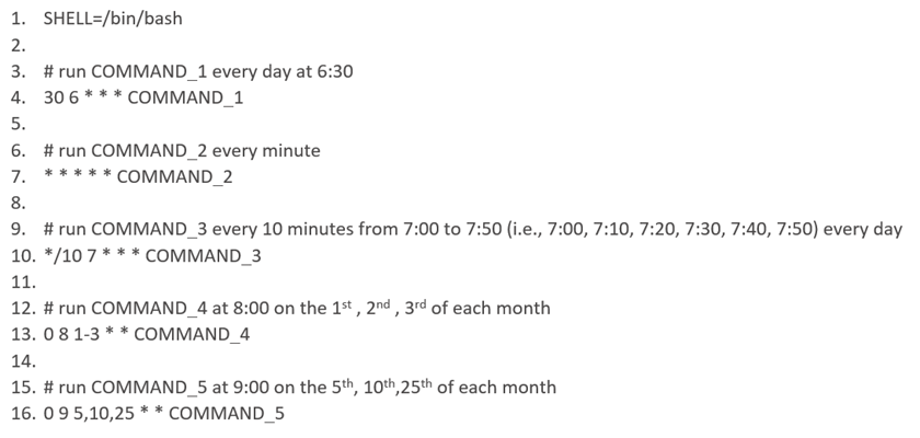
A sample CRONTAB file that schedules a command to be executed every day at 19:00 with descriptions of the time expression. This command executes a script and writes the output to a log file. The first line in the sample CRONTAB file specifies a shell to use to execute the command. Line 2 is a comment to describe the purpose of the CRONJOB and line 3 is the CRONJOB scheduled.

For each CRONJOB scheduling, the expression at the beginning of the line sets up the time for the command to be executed. There are five parameters separated by space representing the minute, hour, day of the month, month and day of the week. An asterisk (*) meaning “always” can be used so the command will be run every minute, hour, day in a month, month or day in a week, depending on where it is located. Here is a demonstration of a few commonly used expressions for scheduling a CRONJOB.

Publishing with Desktop application (GUI-METHOD)

For users who prefer to work with graphical user interface, using the d3VIEW Desktop application will be the best option to publish the test. Once it is installed on the laptop, we can launch the Desktop application and enter the login information. After we are logged in, we can go to the “plugin” tab and choose “BMS plugin” from where we select the directory where the data is located, type in the information about the test required for publishing and select the publishing options we would like to add. When everything is set, we can click “run plugin” to run the plugin and the published test will appear on d3VIEW in the same way as if they were published in any other methods.

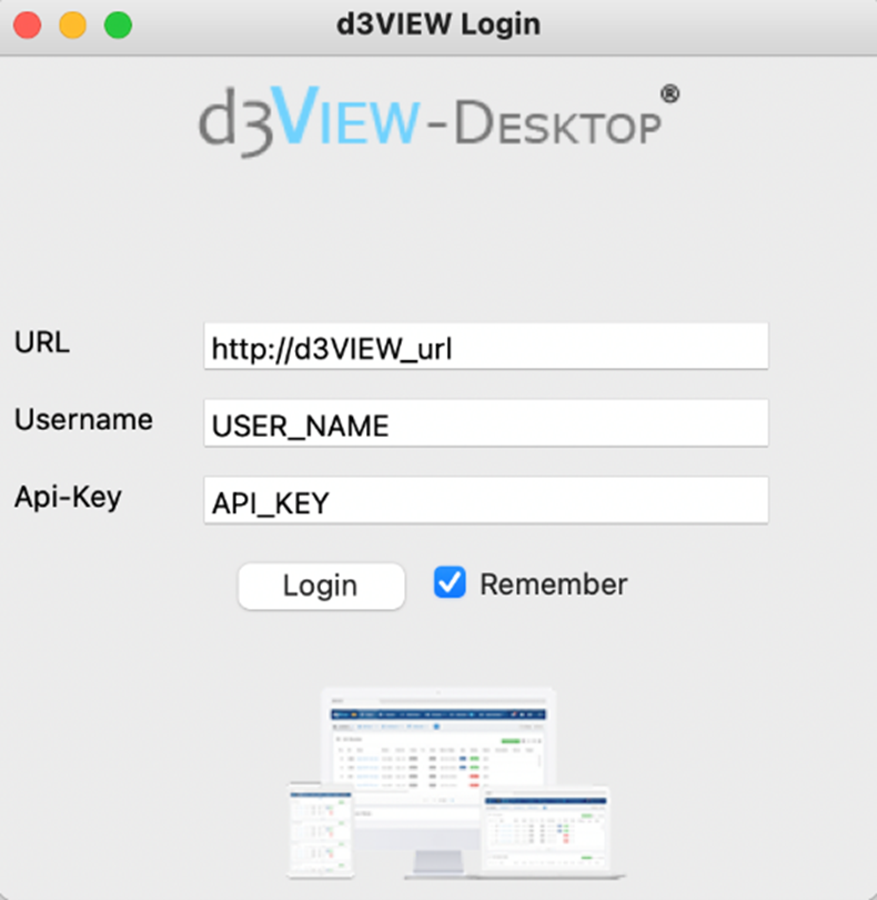
Login page of d3VIEW Desktop application

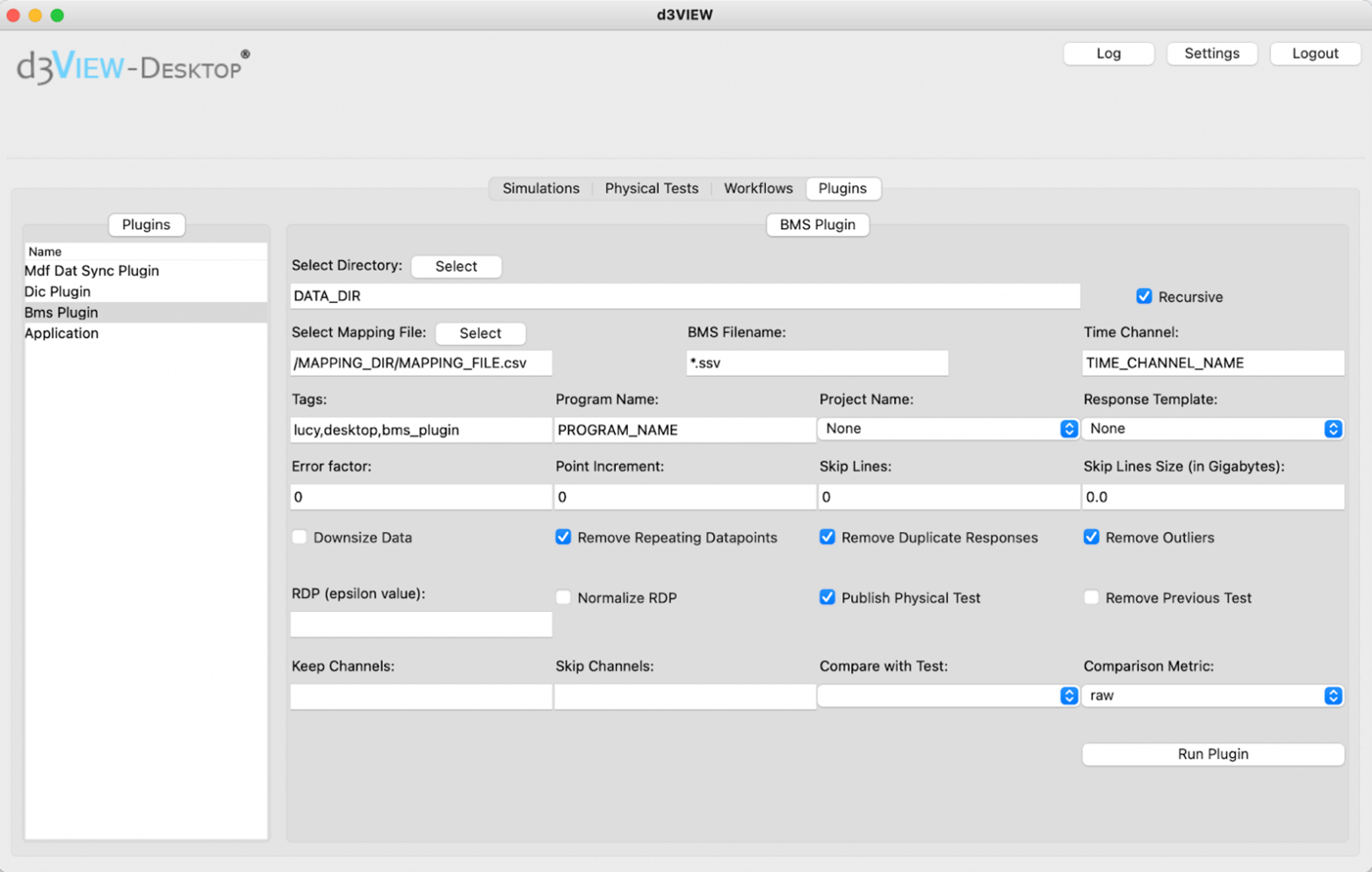
d3VIEW Desktop application user interface. We can choose the directory where the data file is located and check the publishing options and run plugin to publish selected test data.

Mapping File

Besides accurate instructions from the script, a correctly configured mapping file is also a critical component for a successful publishing of BMS test data (Cell data publishing doesn’t need a mapping file).

Signal names from labs	Published names on d3VIEW
Time_Raw_Name	Test Time
Current_Raw_Name	Pack Current
Voltage_Raw_Name	Pack Voltage
SOC_Raw_Name	SOC
SOC_Max_Raw_Name	Maximum Cell SOC
SOC_Min_Raw_Name	Minimum Cell SOC
…	…

The fundamental purpose of the mapping file is to provide instructions on how the source channels to be mapped to d3VIEW channels (which is more standardized and user friendly). Meanwhile, other options from the publishing scripts also requires corresponding configuration in the mapping file.

Basics Structure Of A Mapping File

A mapping file contains rows of mapping records. Each record provides specific instructions on the mapping. One mapping record contains at least 6 of the most basic properties

Basic columns of a mapping file

Columns	Description
Program	Only tests of the specified program will be using the mapping record for mapping. Program is also labelled as “Test Type” in d3VIEW. You can find the test type information from the .wr file for BMS data and from the header at the start of the .csv file for Element and EMEA data.
Source name	The channel name from raw data file, where the dest name maps from. The column names in the data file.
Dest name	The published channel name on d3VIEW the source name will be mapped to.
Source units	Channel units from raw data file
Dest units	Channel units shown on published channels on d3VIEW
Date added	Date when the record is added

We can take the following mapping record at row 3 as an example to demonstrate how the mapping file works. This mapping record will be used for tests from the program “PROG_NAME” only. If the tests being published are from “ABC” or “PROG_NAME_ABC” or “PROG” or any other programs other than “PROG_NAME”, they will not be using this mapping record. To “use” one mapping record is for lucy to look for the source name from the data files and maps it to the dest name. When the test is from the program “PROG_NAME”, it will look in the data file for the column “Current_Raw_Name”, and map it to the dest name “Pack Current”. This means, when the data from that column is published on d3VIEW, it will show as “Pack Current” instead of “Current_Raw_Name” from the data file. This procedure goes the same for the units. “7/28/2021” is the date when this mapping record is added.

Program	Source Name	Dest Name	Source Units	Dest Units	Date_added
PROG_NAME	Test Time_Raw_Name	Test Time	s	s	07/28/2021
PROG_NAME	Current_Raw_Name	Pack Current	A	A	07/28/2021
PROG_NAME	Voltage_Raw_Name	Pack Voltage	V	V	07/28/2021
…	…	…	…	…	…

Many of such mapping records with the same program name forms a mapping table for that program. A mapping file usually contains multiple mapping tables to provide instructions to tests of different programs.

-match-type

As briefly described in the BMS scripts section, the -match-type option provides flexibility on how lucy matches the program name. For example, when tests from programs “PROG_NAME”, “PROG_NAME_ABC”, “PROG_NAME_CDE” share the same. It is tedious to create and maintain duplicate copies of the same mapping table but with different program names. Since they all start with “PROG_NAME”, we prefer to have an alternative way for these programs to use one mapping table. -match-type option provides such feature.

In order to use this feature, we need to provide -match-type option in the script. Meanwhile in the mapping file, we need to add an additional column “Match Type”. In that column, we provide one of the following strings

Match Type	Description
starts_with	Any program with name starting with the program name listed in the program column will use this mapping table.
ends_with	Any program with name ending with the program name listed in the program column will use this mapping table.
contains	Any program with name containing the program name listed in the program column will use this mapping table.
equals	Any program with exactly the same name listed in the program column will use this mapping table.

In the example shown above, all tests with program names starting with “PROG_NAME” (e.g., PROG_NAME, PROG_NAME_ABC, PROG_NAME_CDE, PROG_NAME_EFG, PROG_NAME_GHI) will be able to use the mapping table with program name “PROG_NAME” in the program column.

-use-mse (CrossCheck)

CrossCheck(-use-mse) option provides an additional check for correct mapping by comparing the mapped channels with a “reference” curve we know is definitely correct. To apply this feature, we need to add the following columns:

Columns	Description
CrossCheck	“yes” or “no” to indicate if we want to use CrossCheck feature
CCRef	Channel name we would like to use as a “reference” in the checking
CCT	The metric we want to use for checking. Currently, it supports MSE (mean squared error) method.
CCCriteria	How do we compare the reference metric (e.g., >, <, = )
CCValue	The reference metric we want to compare to.
Alternative	The next candidate to be mapped if the calculated metric using the candidate curve and the reference curve fails the condition set by the CCCriteria and CCValue.

For example, when a candidate curve is selected by the lucy publisher to map to the channel Cell Voltage_###_RAW_NAME, we are calculating the metrics of the MSE between the candidate curve and “Average Cell Voltage”. If the MSE is smaller than the CCValue, that is, the MSE computed using “Maximum Cell Voltage” and “Minimum Cell Voltage”, then we use the candidate curve to map to the channel Cell Voltage_###. Otherwise, we go to the next candidate in the “Alternative” column, CellVolt_###_RAW_NAME. Then, we perform the same check until we find the correct candidate or when we reached to the end of the mapping table or when the “Alternative” is “NONE”.

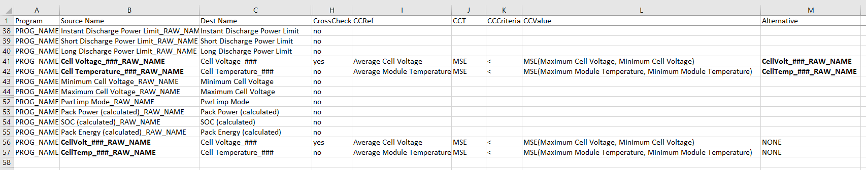
A mapping file with additional columns for CrossCheck feature (-use-mse)

-use-mapper

-use-mapper requires the same columns as “CrossCheck”. But we can put “no” to all items in the mapping file. This option intends to provide a solution in the following scenarios.

• Map source name with a single digit to a dest name with multiple digits. For example, the source name “CellVolt_2” will be mapped to “Cell Voltage_2” and “CellVolt_10” will be mapped to “Cell Voltage_10”. When we order them alphabetically, “Cell Voltage_10” will appear before “Cell Voltage_2”. This is not what we want. So, we need to map “CellVolt_2” to “Cell Voltage_02” if the max number of the Cell Voltage signals are two digits or to “Cell Voltage_002” if the max number is three digits.
• Allow more than one source names in one cell separated by coma. Some tests have different channel names. However, they are from the same program. Channels from one files have this prefix “PREFIX_”. To accommodate this characteristic, we put both channel names to the source name separated by comma. This allows lucy the publisher to look for the second channel is the first doesn’t exist in the data file to map to the dest name.

Program	Source Name	Dest Name
…	…	…
PROG_NAME	Current_Raw_Name, PREFIX_Current_Raw_Name	Pack Current
PROG_NAME	Voltage_Raw_Name, PREFIX_Voltage_Raw_Name	Pack Voltage
…	…	…

Downsampling

Downsampling methods help to reduce the number of points from the raw data without losing information of the original signals or lose as little information as possible. There are several methods available to achieve this with lucy options in the publishing script. #. -rm-repeating #. -error-factor #. -rdp

-rm-repeating

The option -rm-repeating removes points having the same values as their adjacent points both on the left and on the right. Therefore, -rm-repeating the size of data without losing any information.

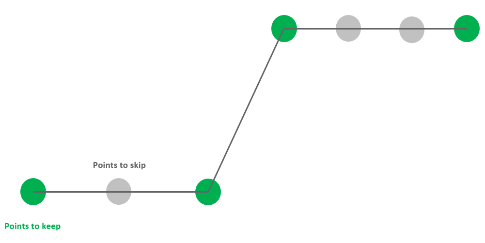
-rm-repeating removes points having the same values as both adjacent points.

A simple example before (blue) and after (red) -rm-repeating is applied.

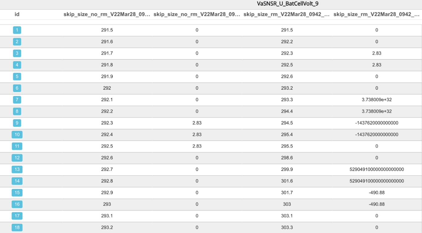
Table view of signal published with (right) and without (left) -rm-repeating option option.

This shows how the -rm-repeating works by listing the x and y values from the raw data (left) and simplified data (right) side by side. Clearly the first 2 points from the simplified data doesn’t contain any less information than the first 8 data points from the raw data do, only with fewer points. This can be verified from the line view of these two curves.

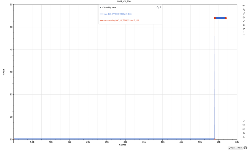
Line view of the signal published with (red) and without (blue) -rm-repeating option

The two signals, red published with -rm-repeating and blue published without -rm-repeating, match each other perfectly. This confirms that -rm-repeating doesn’t discard any information from data in the down-sampling procedure.

-error-factor

-error-factor is one parameter for the -rm-repeating option. It removes points with the following condition. If \(abs(y_{prev} – y_{curr} )<\) error factor \(×(y_{max}-y_{min})\),then \(y_{curr}\) is dropped.

We always keep the first and last point of the curve. Then, we examine each point starting from the second point of the curve. It determines a tolerance value by taking a proportion (error factor value provided by user) of the y range (difference between max and min y values of specific signals). If the current point is outside of the tolerance, then both the current point and the previous point will remain. Otherwise, if the current point is within the tolerance, it will be skipped unless the point after exceeds the tolerance.

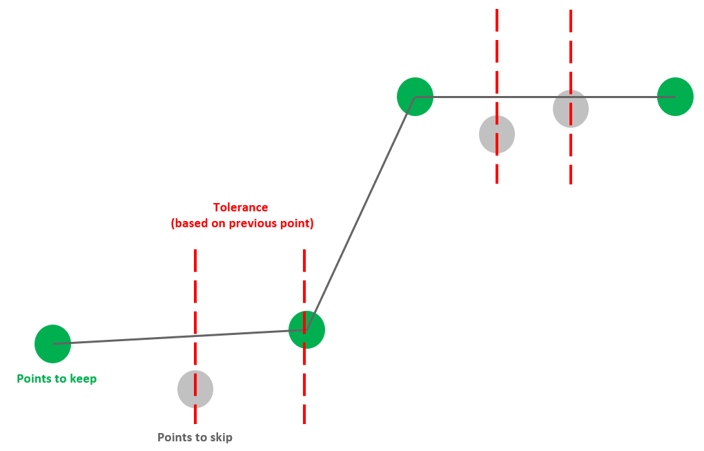
-error-factor removes points having the “similar” values as both adjacent points.

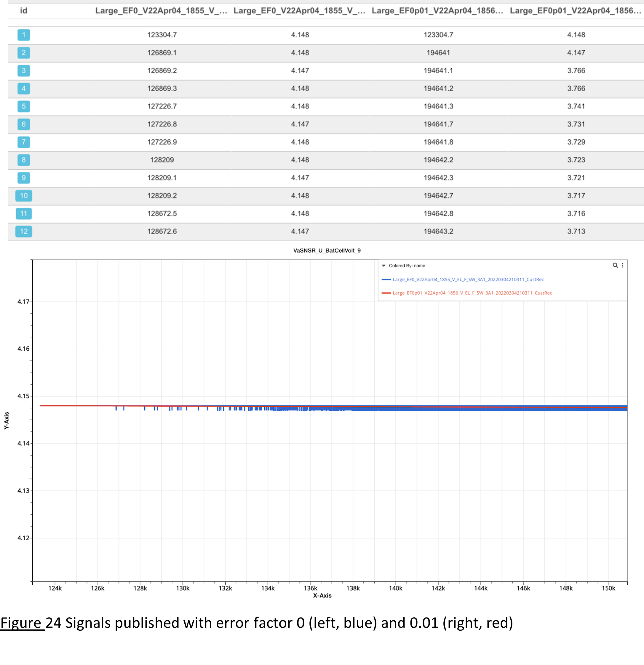
Signals published with error factor 0 (left, blue) and 0.01 (right, red)

Two signals published with different -error-factor values 0 and 0.01. First a few points from the raw data are all around 4.147 but varies by 0.001. In this case, -rm-repeating will not remove these points because they have different values. However, variation of size 0.001 may be not of our interest compared with the y range of the signal being about 1 (ymax = 4.148, ymin = 3.144). When the -error-factor is set to be 0.01, then if the difference between two adjacent points is less than 1% (-error-factor 0.01) of the yrange (i.e., 1), then the points are dropped. Thus, -error-factor simplifies the raw data by making a small compromise of the information preserved in the publishing process.

-rdp

The Ramer–Douglas–Peucker algorithm is an algorithm that decimates a curve composed of line segments to a similar curve with fewer points. It is similar to -error-factor in the sense that, it takes an epsilon value that later will be used as a tolerance to determine if a point will be removed or not. Figure 25 shows the simplified signal with epsilon value 1 and 0.2. Smaller epsilon value leads to fewer points dropped and therefore, there always exists such an epsilon value whose simplified data are close enough to the raw data.

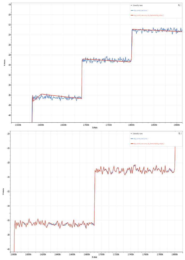
Simplified signal (red) with epsilon 1(top) and 0.2(bottom)

One way to reduce the effects of the scale on the rdp method is to use -normalize option to normalize the raw data using min-max normalization to a 1 by 1 box and then perform rdp algorithm. In this way, the variation in the optimal epsilon values for different data is much less.