6. Simulations
As scientists and engineers, we all know the importance of simulations in solving complex real-world problems safely and accurately. Simulations make information and data conveyable for better decision-making. d3VIEW provides the ability to manage, create, track, compare and share your simulations and their data more effortlessly and efficiently. The Simulations application is divided into four main parts: Preview, HPC Job, Files and Responses. In this tutorial, we’ll review navigating the home page and these sections, so you can start managing your simulations more effectively.
What Will Be Covered
- My Simulations Page
- Preview and Simulation Details
- Errors and Warnings
- HPC Job
- Simulation Files
- Simulation Responses
6.1. My Simulations
From the d3VIEW home page, click on the Simulations button in the left side panel to go to the Simulations main page.
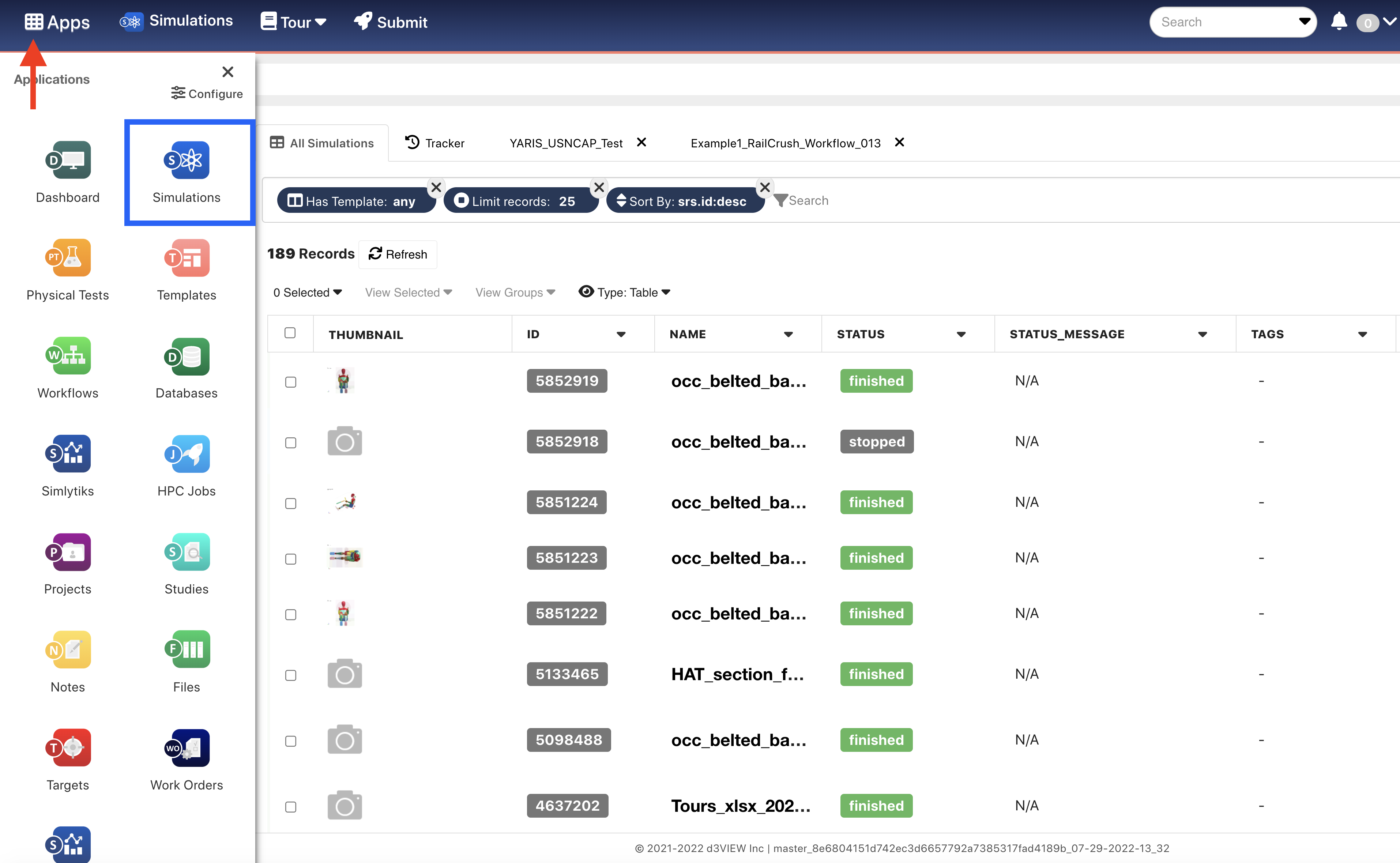
Figure 1: Accessing Simulations
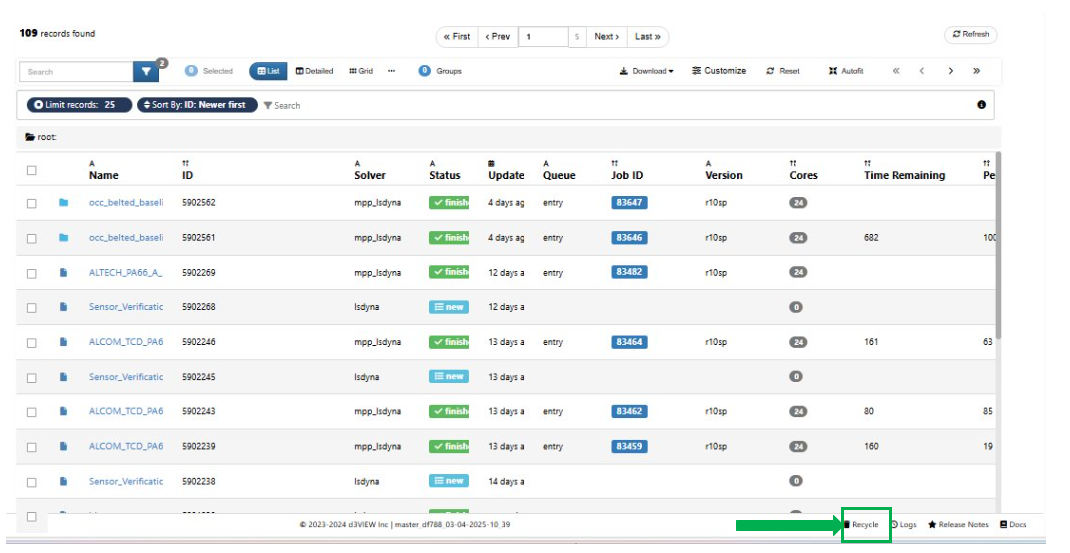
Here, you can submit a new simulation (1), sift through your simulations by using the quick filter buttons (2) or using the drop down or search bar in advanced filtering (3). Review and restore any of your deleted simulations at the bottom by clicking on Recycle (4).
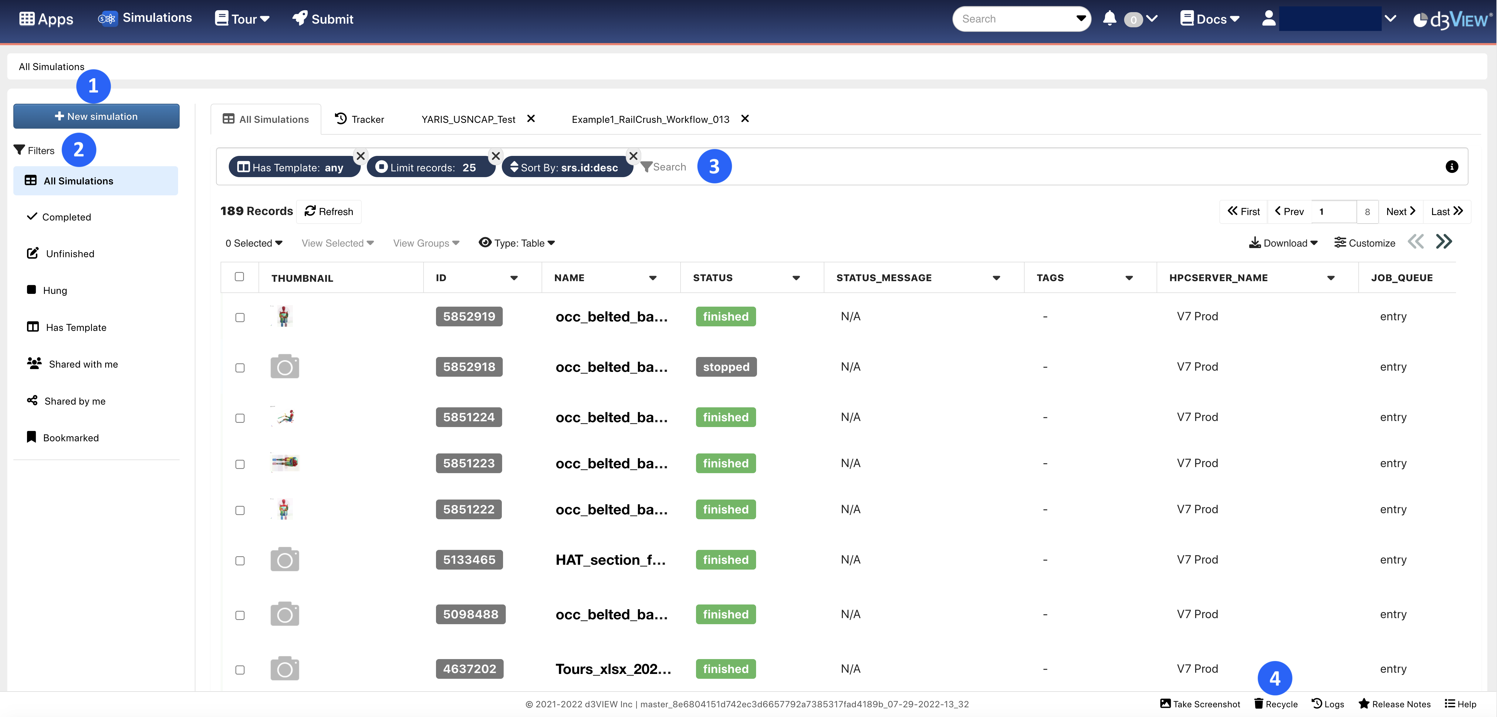
Figure 2: All Simulations
We can utilize advanced filters when we want to look for specific simulation qualities such a solver type or termination type as demonstrated in the following video:
Simulation Home page
Revamped the Simulations page with modernized summary cards for improved clarity and usability.
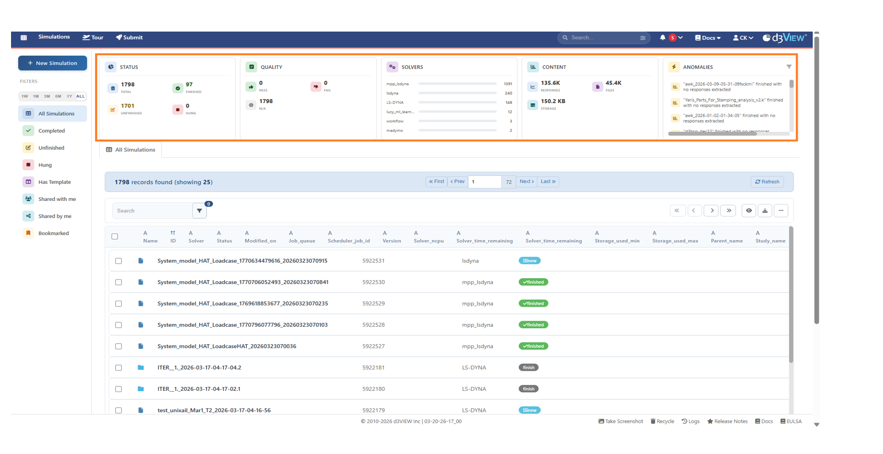
All Simulations
Added draggable summary cards, allowing users to reorder them based on preference
Simulations home page
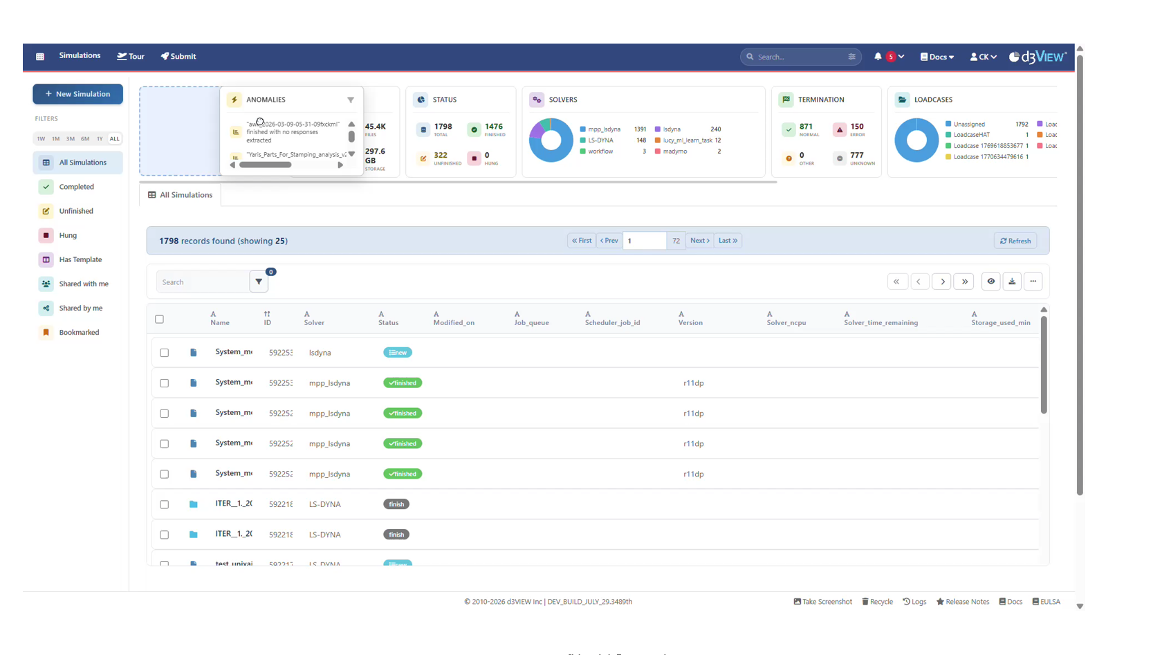
Simulation Summary Card Visibility
The Simulation Summary cards now dynamically adjust their visibility based on user navigation within the Simulation view.
Overview
When navigating between the main table view and individual simulations, the visibility of Simulation Summary cards is automatically managed to improve focus and usability.
Behavior
- Simulation Summary cards are hidden when a user navigates to a specific simulation.
- The cards automatically reappear when returning to the main table view.
- Existing toggle controls are preserved and continue to function as expected.
Benefits
- Reduces visual clutter when working within a specific simulation
- Improves focus on detailed simulation data
- Maintains user control through familiar toggle functionality
6.2. Simulation Preview
UI for home tab of Simulations that are submitted completely is updated.
Home tab updated
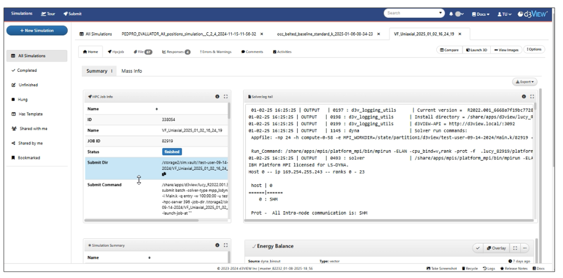
Click on a simulation in the list to open and see its contents in a new tab.
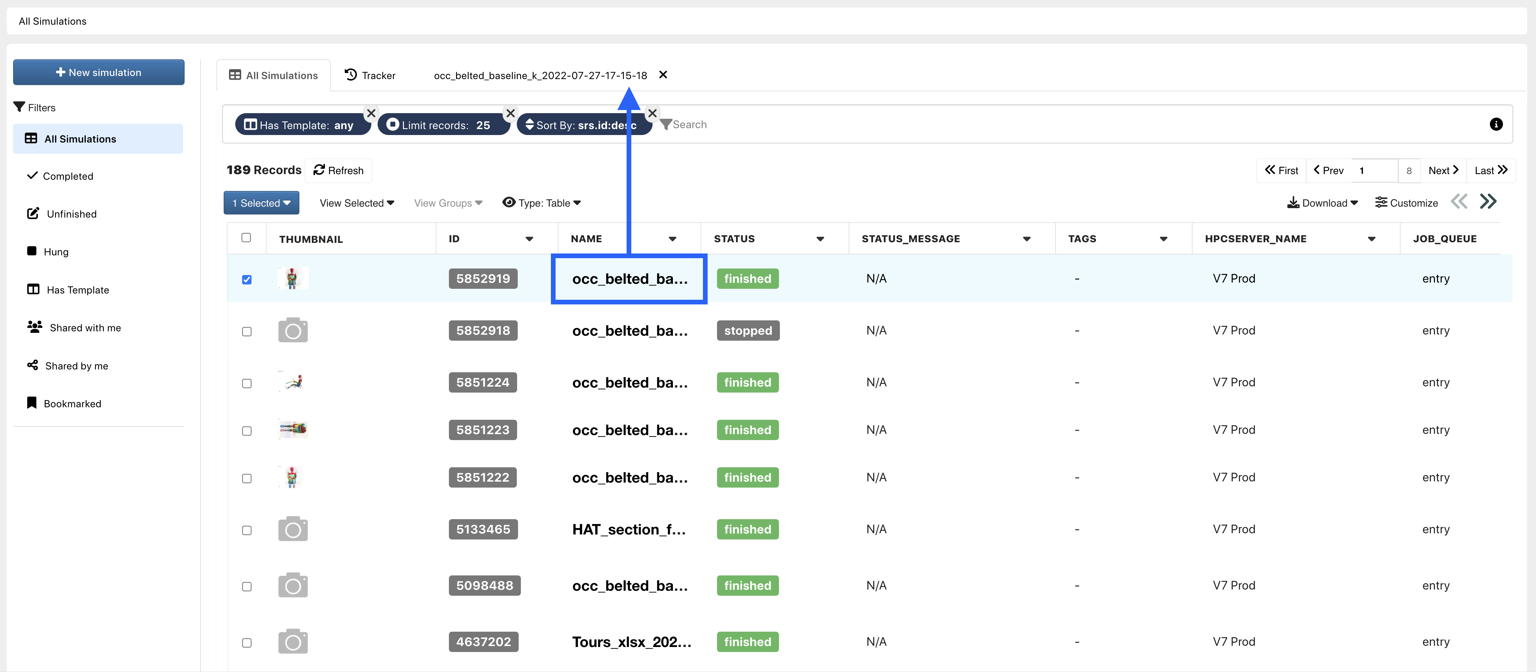
Figure 1: Open Simulation Viewer
The first section at the top, ‘Home’ provides a real-time status of the simulation while it is running. The panels allow you the visualize different elements of the running job. Some useful information to examine are energy balance, minimum time-step history and time remaining for completion. Energy balance provides incite into detecting any abnormalities in the simulation and, if required, kills it before the end time. You can also click on the last section ‘Errors and Warnings’ to identify any issues with the simulation.
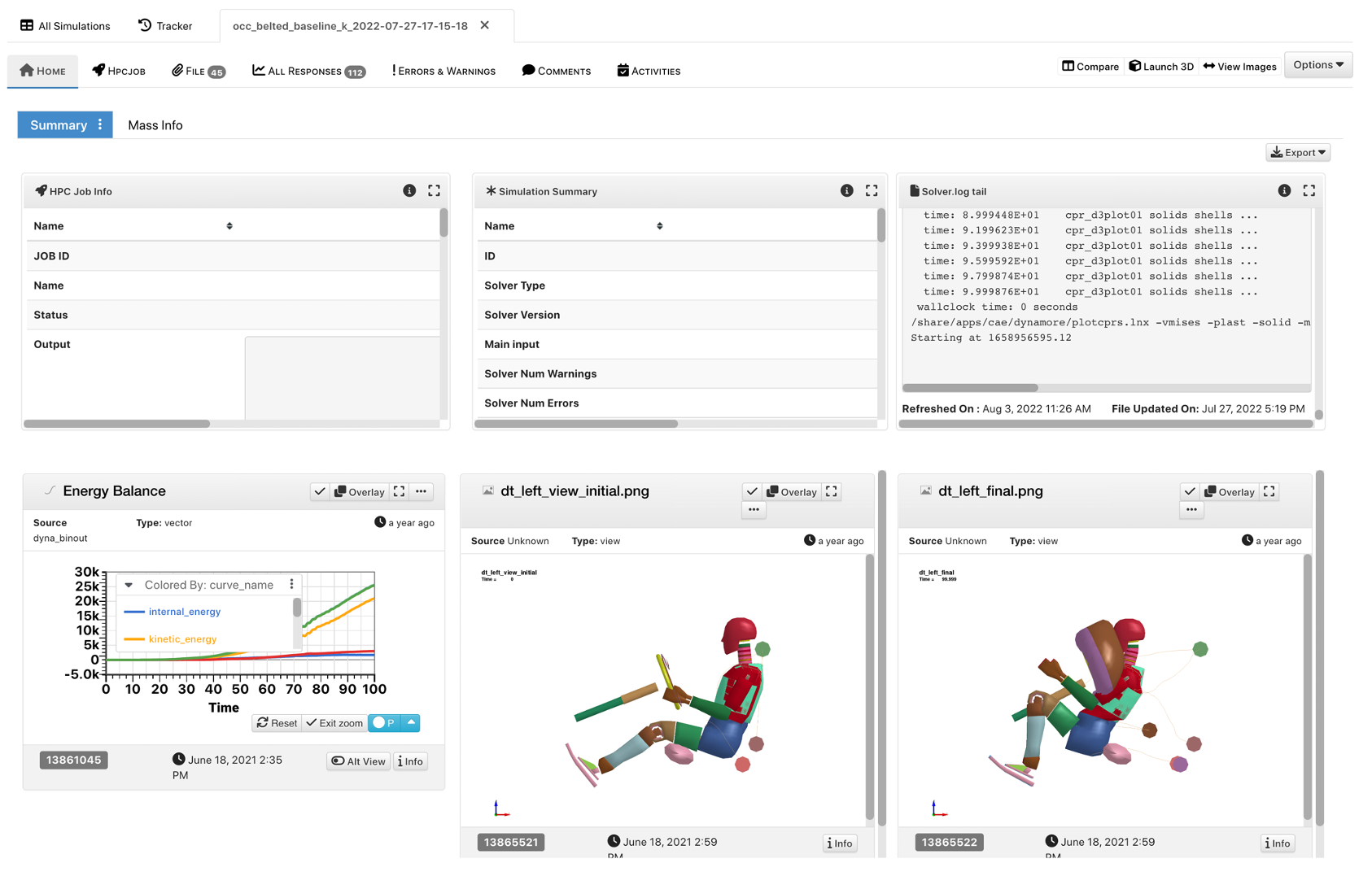
Figure 2: Simulation Details
Simulation Processing Statuses
Here is a graphical representation of the processing statues a simulation runs through while solving:
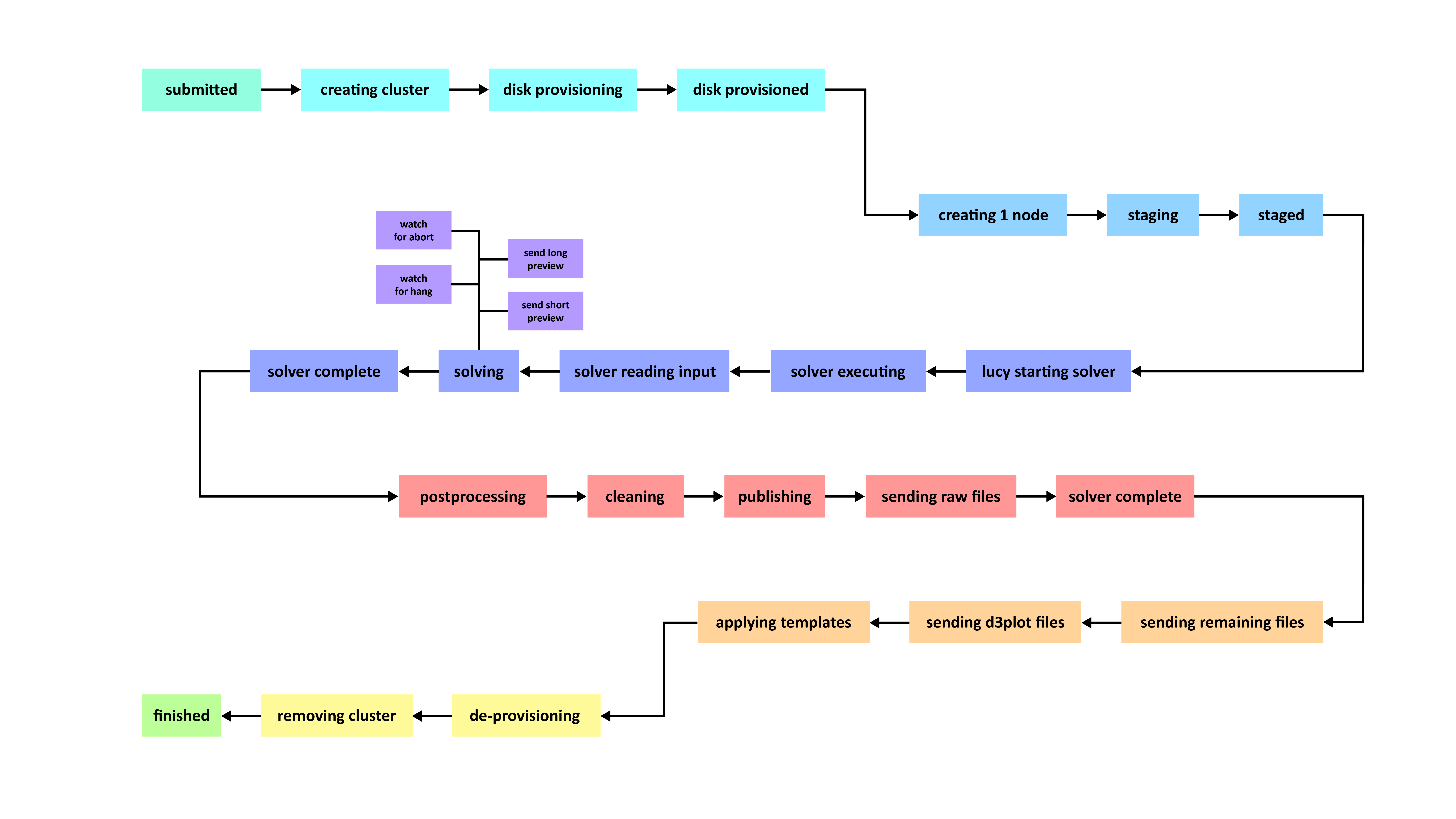
Figure 3: Simulation Processing Statuses
6.3. Simulation Errors and Warnings
View all the errors and warning from simulations files under this tab in your simulations. This reduces the need of searching for errors in your simulation files.
Figure 1: Simulation with No Errors or Warnings
Email Notifications
If you have an email linked to your account, you’ll also receive warning and error messages once the simulation is done solving via email. To update your email, click the down arrow under your name at the top right corner of the screen (1) and choose ‘Settings’ (2). Then under ‘Info’ (3), input your desired email in the space provided (4).
Figure 2: Update Email
Here are some examples of email notifications we may get of errors in our simulations
Figure 3: Email Notification Examples
6.4. HPC Job
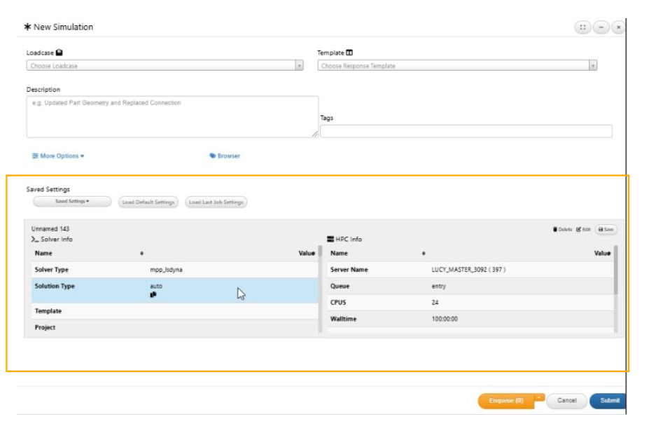
In order to run a simulation on the HPC, you have to submit a job. To start a new job submission, click on ‘New Simulation’ in the upper right corner of your Simulations page and follow the instructions presented in the previous tutorial section: Job Submission. Submitting a job requires a specified configuration which can be reviewed after clicking on the respected simulation and going to the HPC Jobs tab at the top. This tab provides the job submission history such as the node the job was submitted to, the number of CPUs used, etc. The information can be useful as comparisons and guides for submitting new simulations.
Figure 1: HPC Job
Settings table
Saved configurations while submitting a simulation are now shown in a table format.
HPC settings table
6.5. Simulation Files
Simulation files are processed through the server and compute node to be available to you locally.
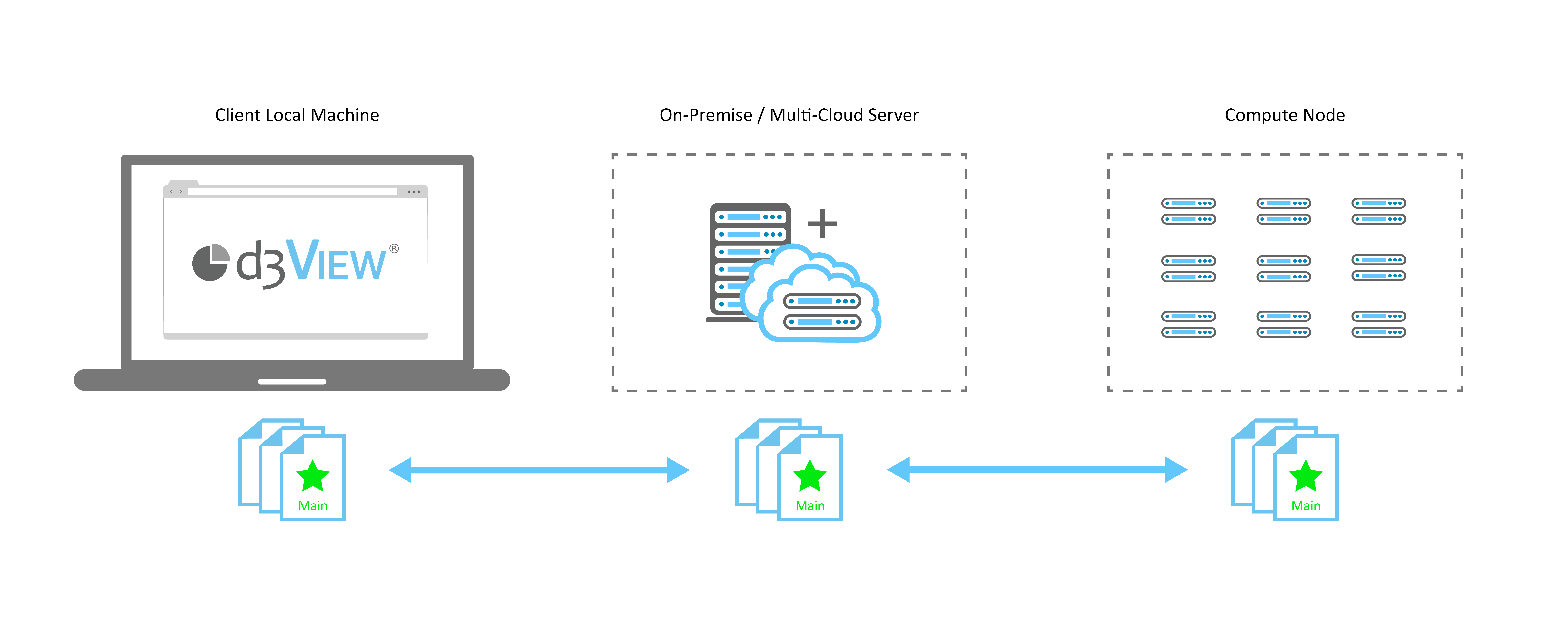
Figure 1: Client-Server-Compute Node File Location
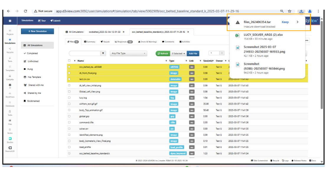
All the output and log files generated by the solver (bin-outs, d3plot, solver.log etc.) are available in the Files tab (1). Download, share or view individual files by clicking on the 3 dots next to it (2). Add a new file at the top (3).
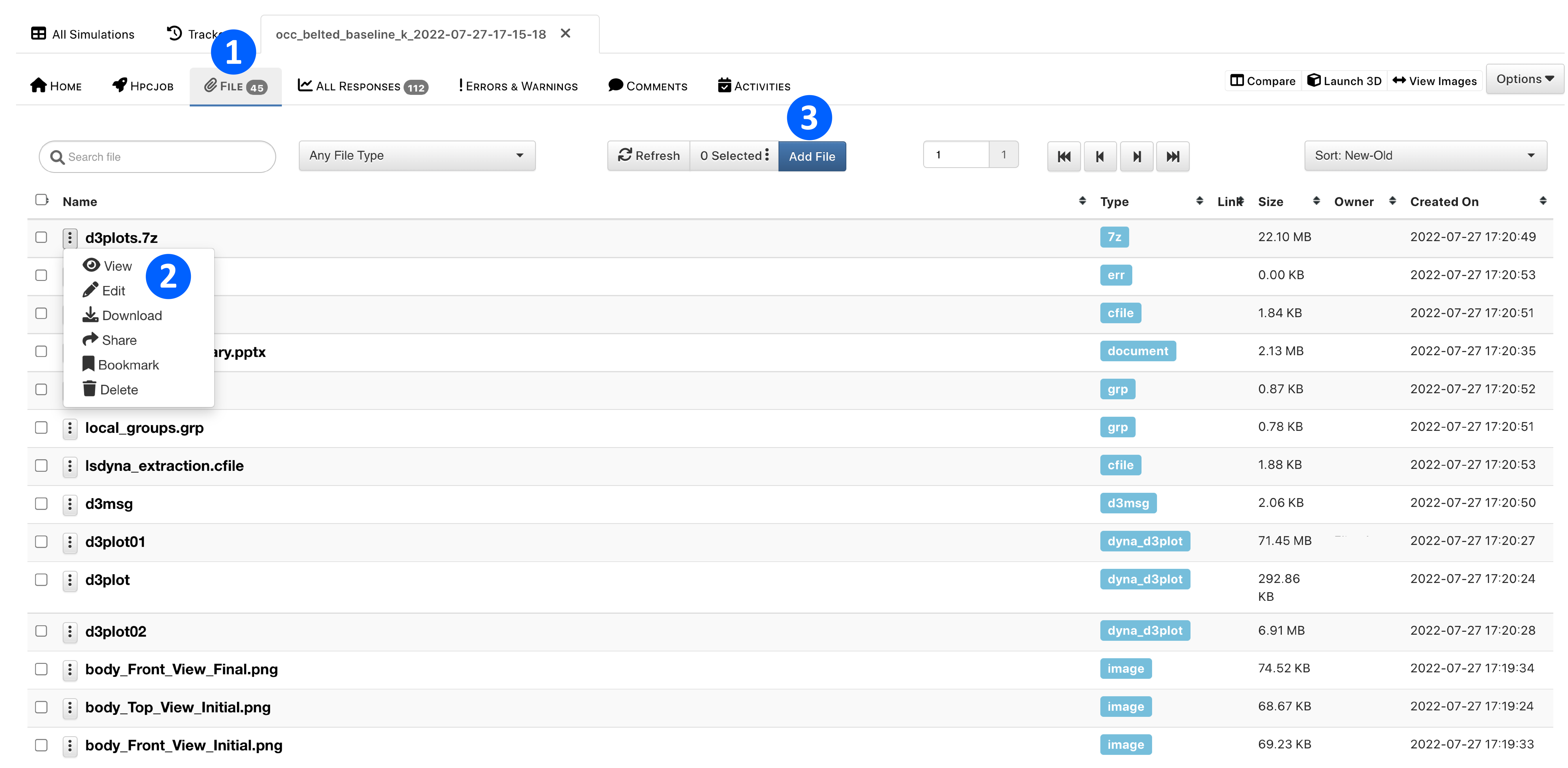
Figure 2: Simulation Files
Viewing a file opens it in another window that is adaptive to the file type. Here, you can review the file by utilizing the search bar (1) or download it (2).
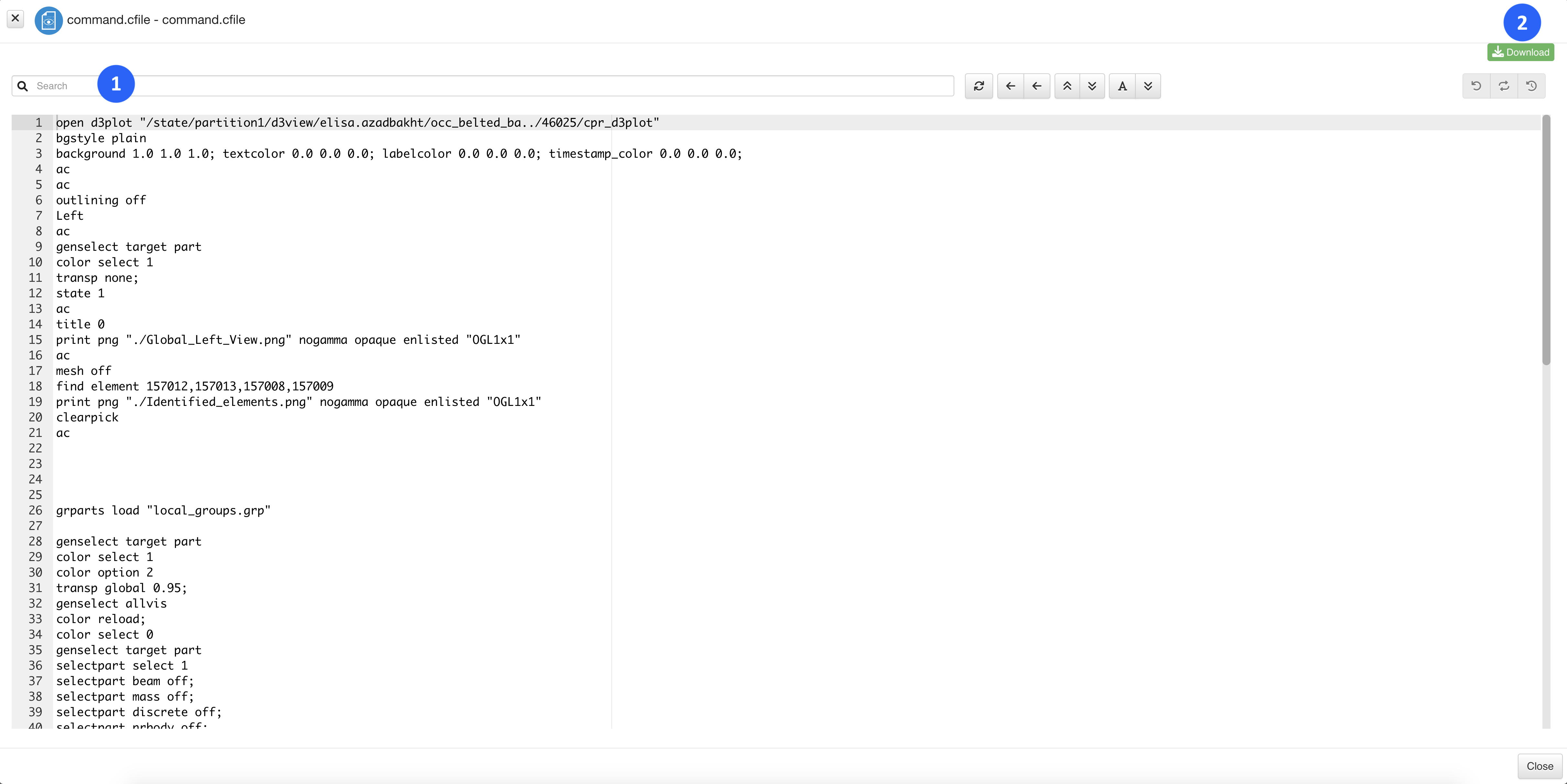
Figure 3: File Viewer
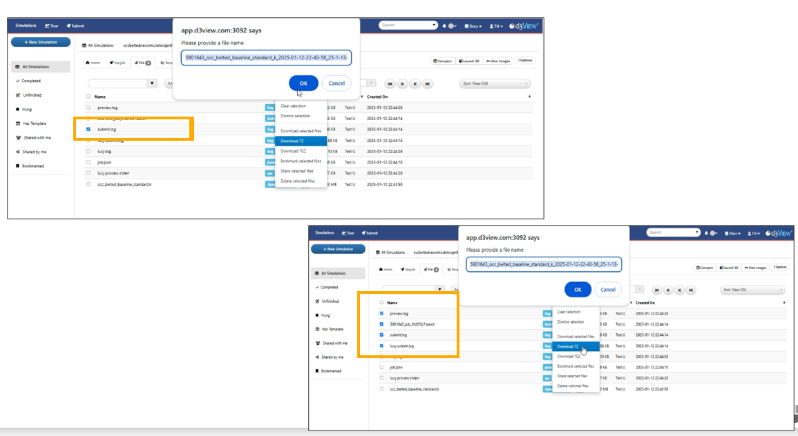
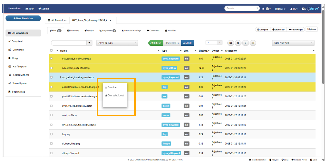
Download or share multiple files at once by selecting them via the checkmark (1) and using the Selected drop-down menu (2).
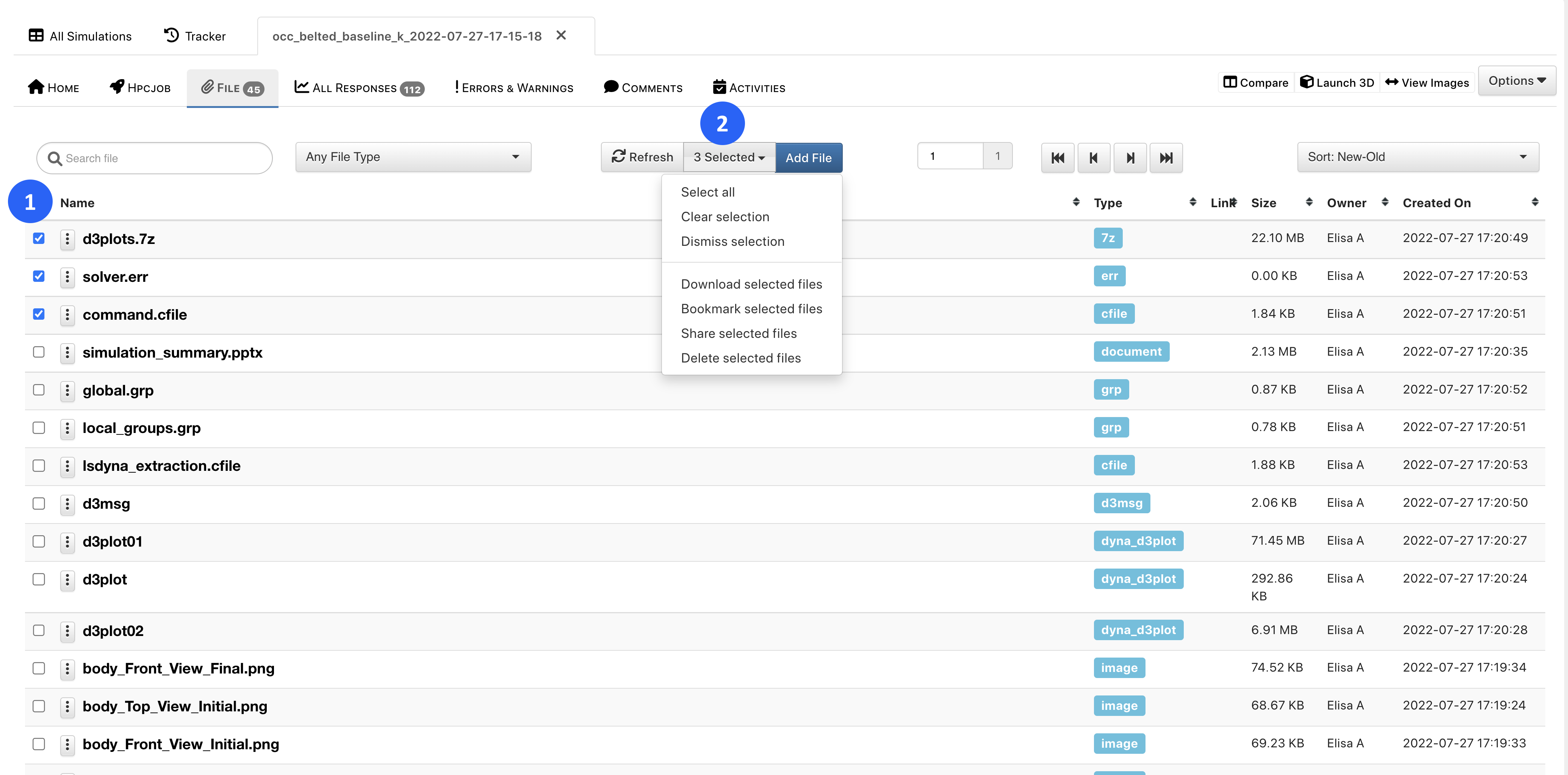
Figure 4: Multiple Files Actions
New as of October, 2022, the data viewer supports JFIF images as shown in the following image.

Figure 5: JFIF Image Support
We can now specify the name of the file exported when exporting multiple files from the Simulation/Files.
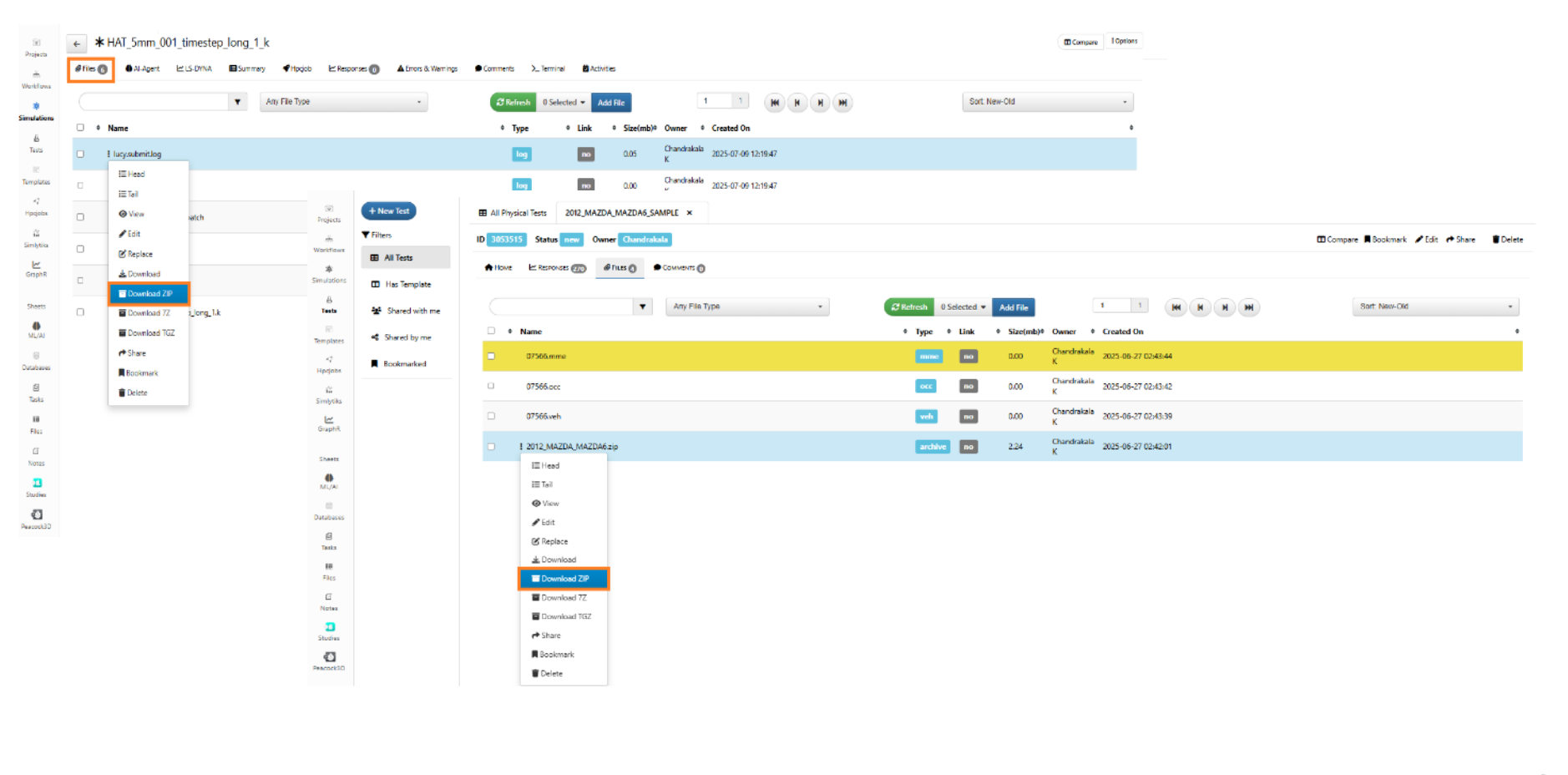
File downloads now support ZIP format for Simulations and Physical Tests.
Download Files
Transform
Files in Simulations/Physicaltests have new option called ‘Transform’ using which we can add translator, path etc., before uploading them to the files tab.
File Watcher
You can watch files in Simulations using File Watcher which has options to refresh the timer and url. They following video shows an example:
Lucy Log
You can view lucy.log files for simulations and visualize the rate of communication between Lucy and d3VIEW.
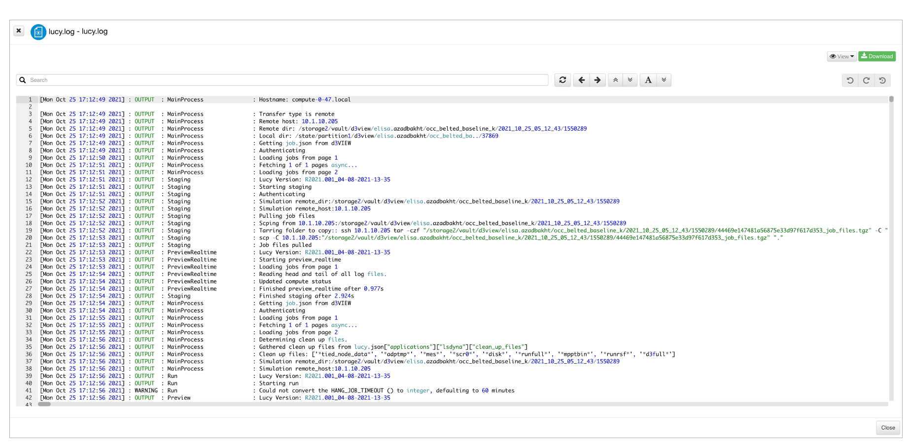
Figure 6: Lucy Log
You can also change view type to log nester for lucy.log files which groups the aspects such as OUTPUT and ERROR.
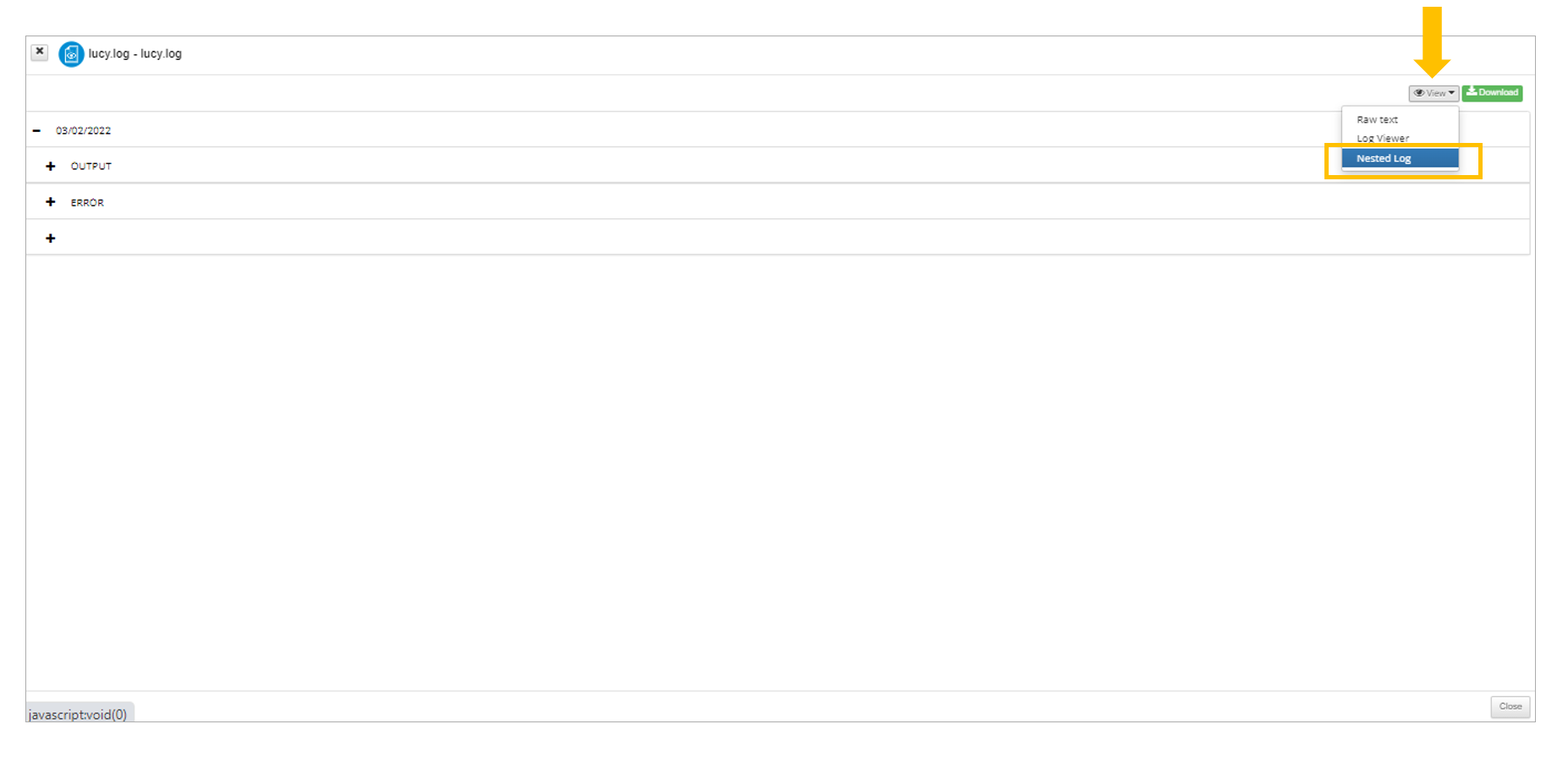
Figure 7: Log Nester
Excel files peacock
Peacock 3D UI is updated similar to Workflows page with controls at the top right, maximize button at the top right, slider at bottom center and nav menu items on the left.
Peacock 3D UI
Excel based ZIP is now supported in files which contain the geometry for nodes, elements etc.
Excel based Geometry
New format of geometry.xls peacock file is now supported in Files to construct a model.
3D Peacock fringe now supports a new option within its legend to color the parts based on difference between the states.
Export
Single and multiple files in the Simulation can now be exported in ZIP/TGZ/7Z formats.
Export files
The default attachment download is updated to export a TAR file.
Export files
The Simulation files with specific types can be exported. The type will be included in the downloaded ZIP file.
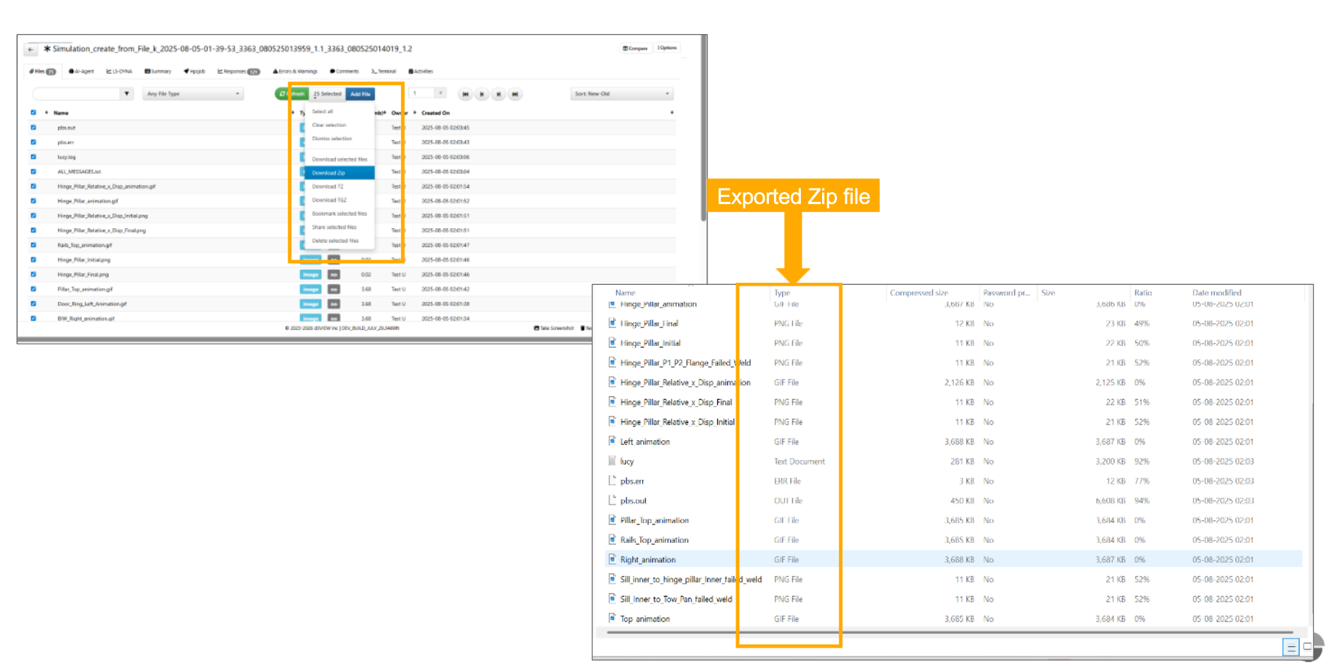
Export files type
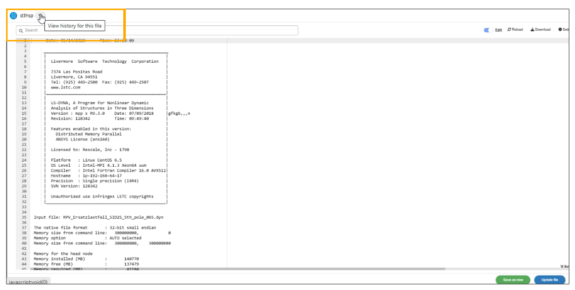
Editing files
Files can be edited and saved as a new file or updated to the same file in Simulations.
Files list in the Files editor is shown in the top right of the header as a simple dropdown list.
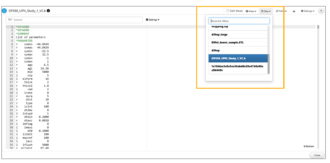
Files List
The text file inside the ZIP in files tab can be edited and saved using save file edits option. The files edited can be saved as a new ZIP file using save as new file option in footer.
History button is now available next to the name of the file in data viewer
History in Editing files
the original and the current pages side by side, highlighting the changes made to the file.
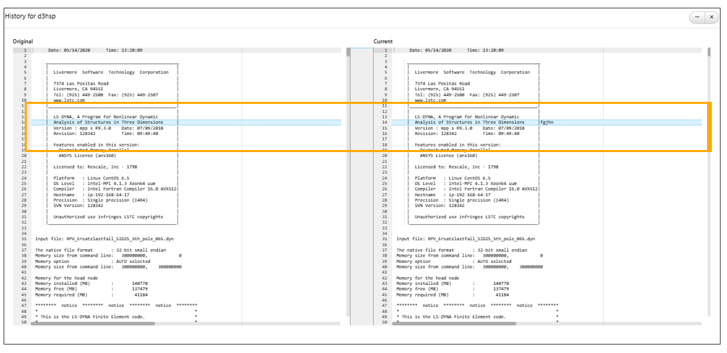
Original and the current pages side by side
The context menu options are now available for the files in the Simulation.
Context menu options
The Files dropdown that is available upon opening a simulation will list all the files available withing a simulation. Any of these files can be viewed by selecting/switching to it.
6.6. GREP Mode
File viewer in Simulation files tab will now show the VI and GREP mode when the file is opened in edit view.
6.7. Simulation Responses
Data output extracted from the simulation and its bin-outs, d3plots (nodal displacements, element_history, etc) are available in the Responses section (1). Any top, front and left view animations are available by default. Use the View Type and search bar (1) or the quick filters such as the image button (2) at the top to search through your responses.
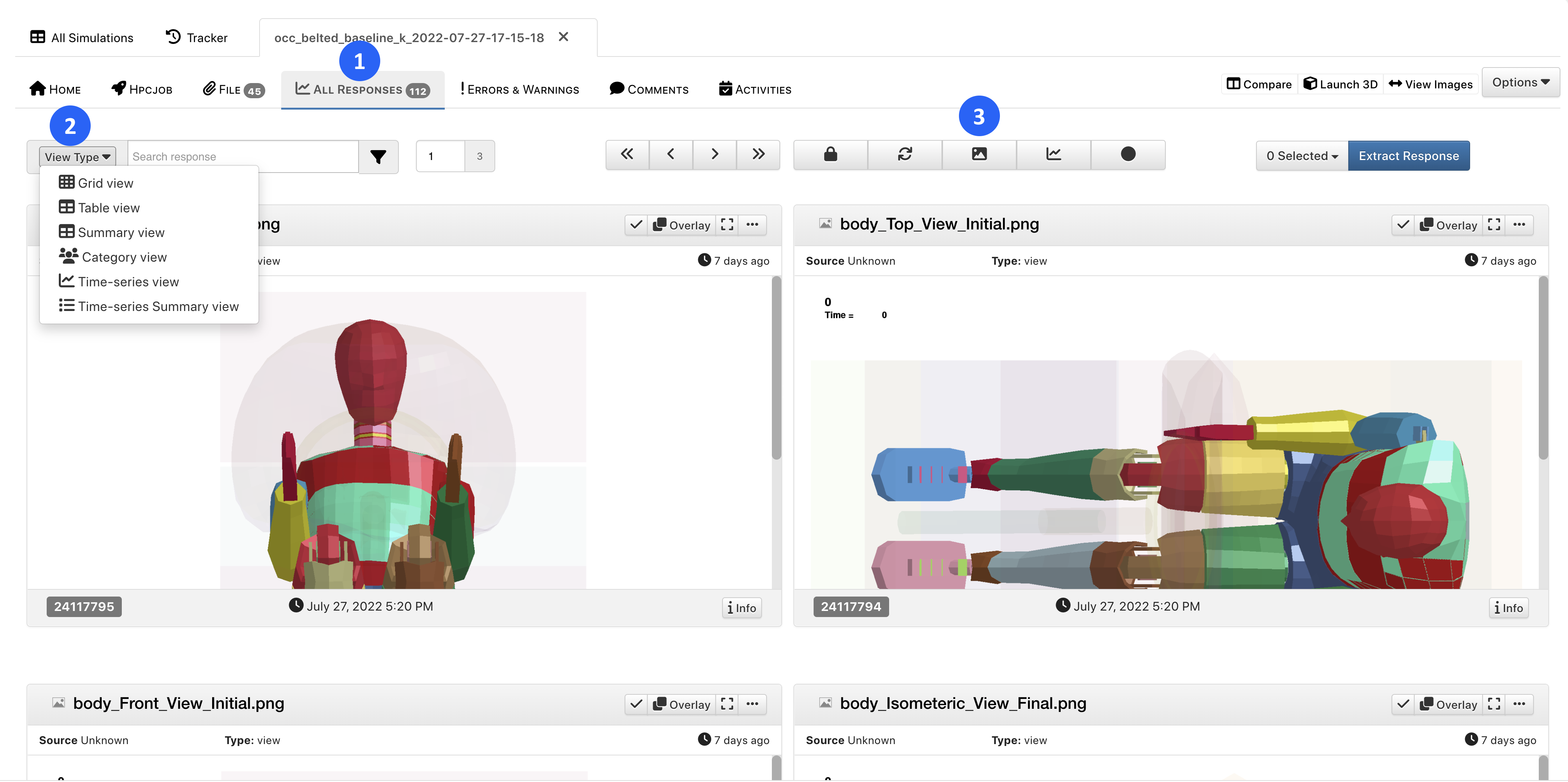
Figure 1: Simulation Responses
You can perform actions on a single response (1) such as viewing in full screen, exporting, sharing or duplicating it. You can also perform actions to selected responses from the drop-down menu (2) such as creating a template from the responses or exporting them to PowerPoint.
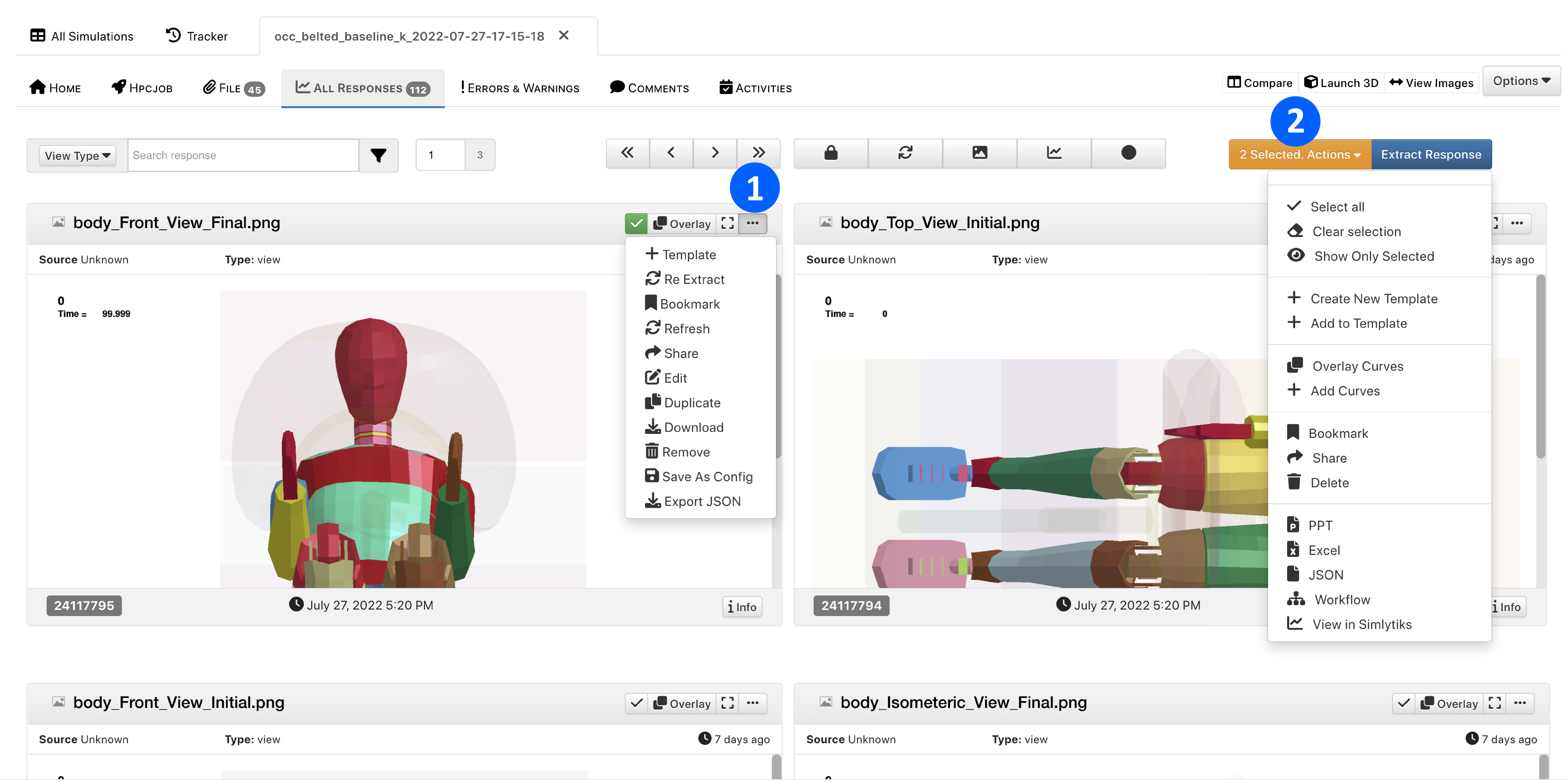
Figure 2: Response Actions
Add a new Response to your simulation by using the data extraction tool.
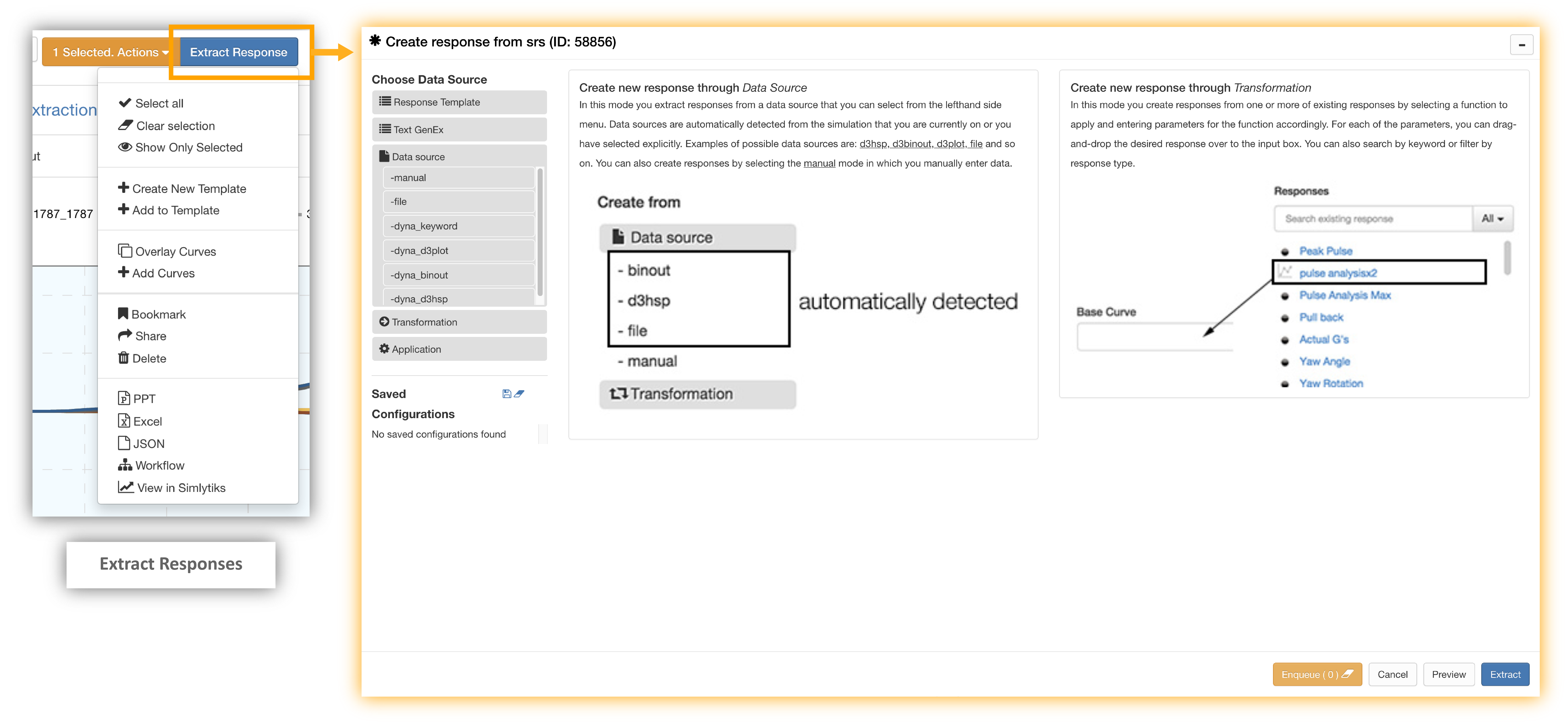
Figure 3: Extract Responses
Curve Responses link with d3VIEW’s Curve Viewing Application Newton for enhanced analysis. To learn about Newton, follow this link.
View Images
Use the View Images button to quickly view images in a simulation.
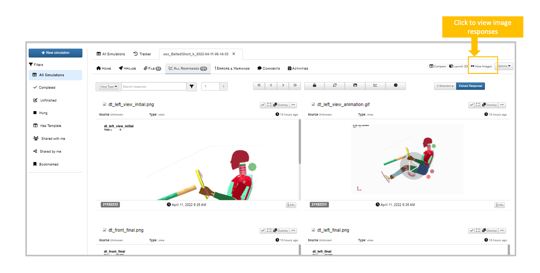
Figure 4: View Images
Filtering
Click on the filter icon at the top to use customized filters for sifting through your simulation responses.
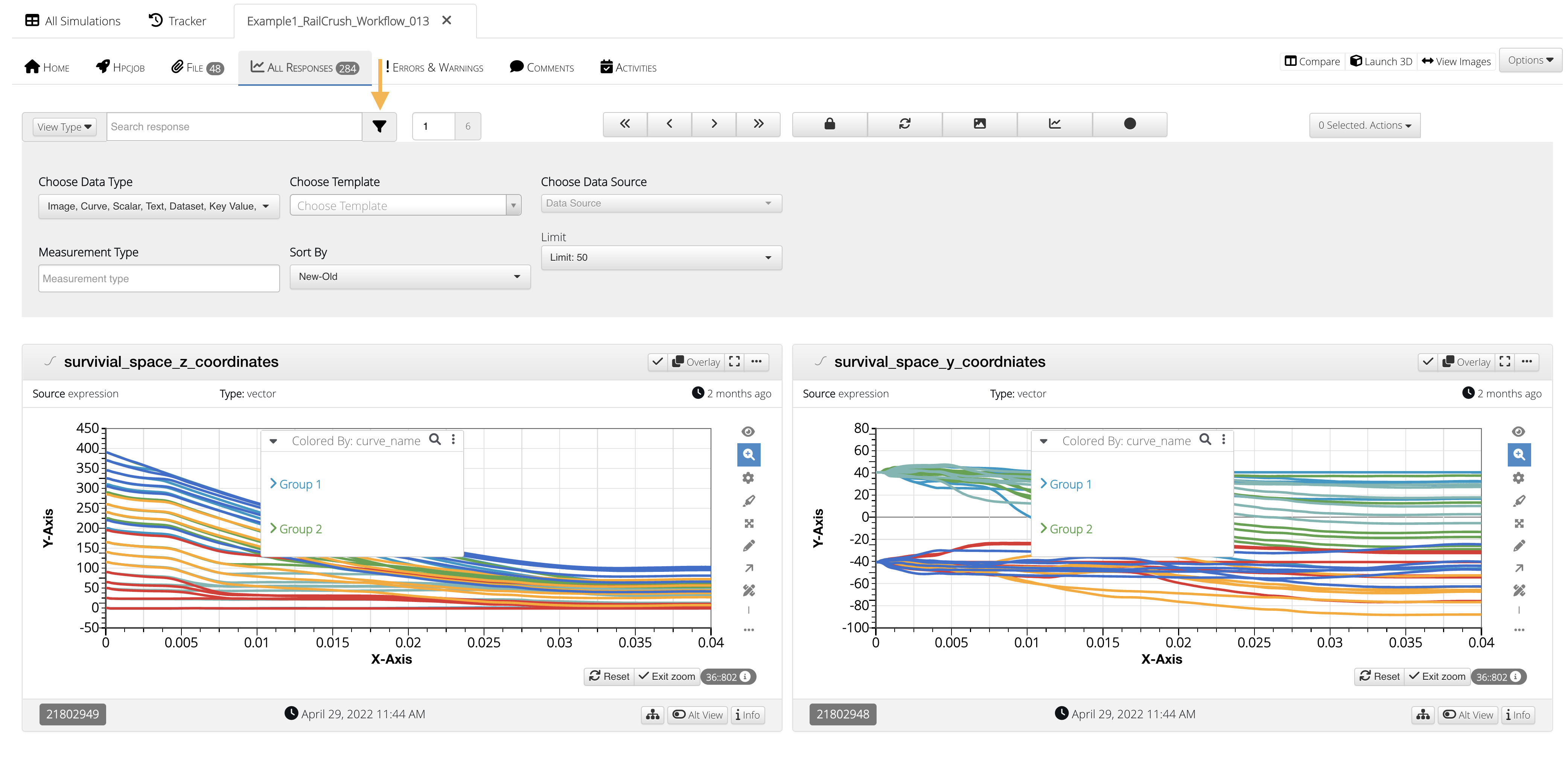
Figure 5: Filter Responses
The datatype filter has an array of filetypes to choose from including MDF/DAT file options which have been adde as of February 16, 2022.
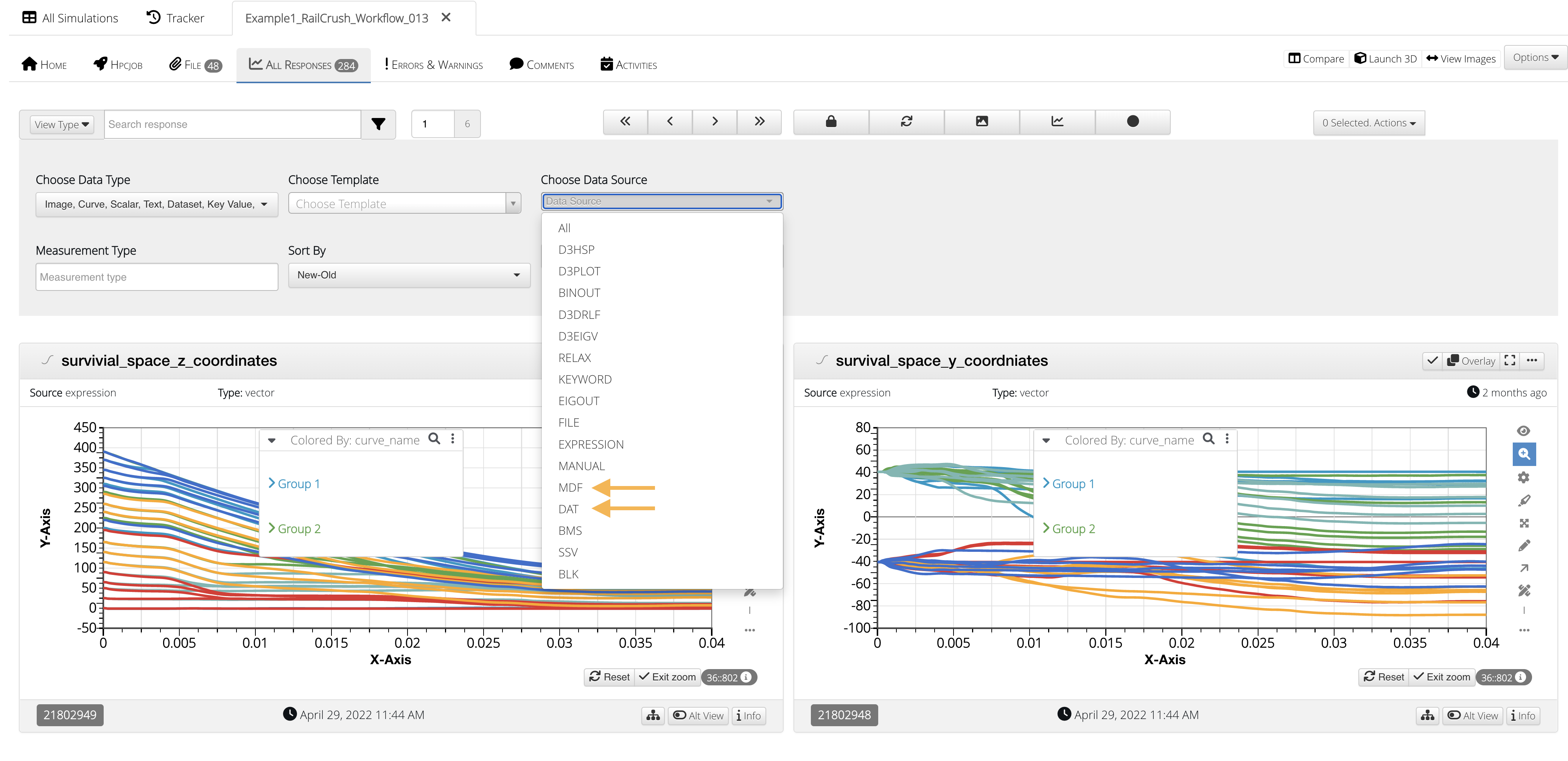
Figure 6: Filter Data Source
Comparing Responses
Simulation responses can be compared in Simlytiks with other simulation or physical test responses. Let’s review
Comparing with a Template
We can compare responses using a template which will have visualizations set up already for us. Watch the following video to see how it’s done.
Comparing with a Template
Comparing without a Template
We can also compare without a template. The following shows how to do this with an example where the simulation is compared with a physical test.
Comparing without a Template to a Physical Test
Compare responses now has an option to set the extraction type to all simulations using a single button at the top.
Add records option available while comparing records of the page now shows filters and records can be selected based on filters.
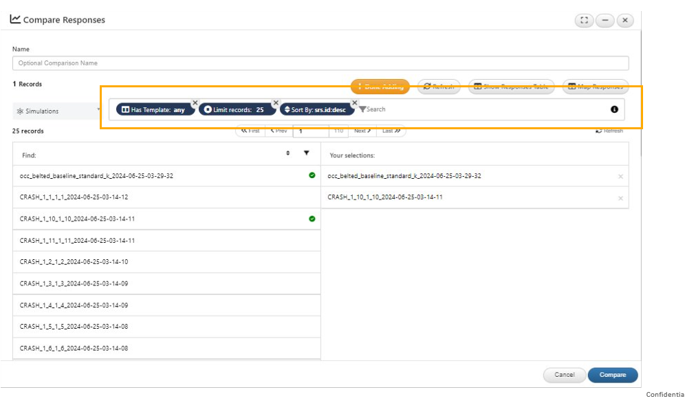
Add Records option
Records selector filters and records can now be sorted and saved.
Added a refresh button in the remote lookup record selector view.
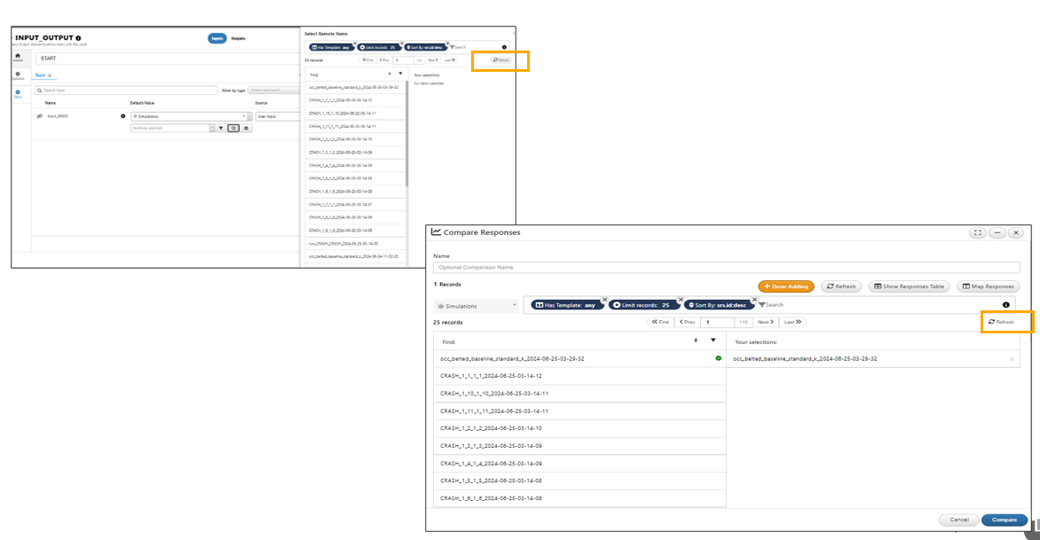
Refresh button
Compare responses option in Simulations/Tests has new option to use Response Extraction Order either in the Dependency Order or Creation Order of responses
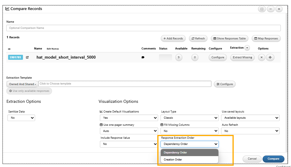
Extraction order
‘Compare Responses’ in Simlytiks has new option called ‘Download logs’ which is available to download logs during extraction in Simlytiks
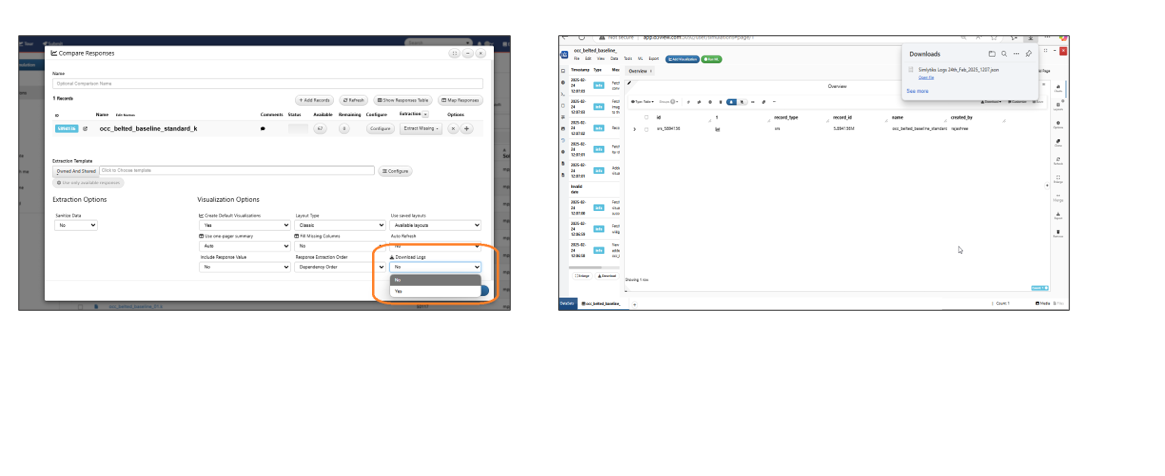
Download Logs
Comapre files
‘Compare Files’ in Simlytiks will now support the responses’ text files to be displayed side-by-side for comparison.
Remote lookup selection
In Compare Response window in the record selector list, We can click on the link icon (remote lookup selection) to view the selected Simulation/ Physical tests records.
Responses updates
CURVES_FILTER/CURVE_FILTER worker in responses now has time scale factor options 1.0 (sec) and 0.001 (sec)
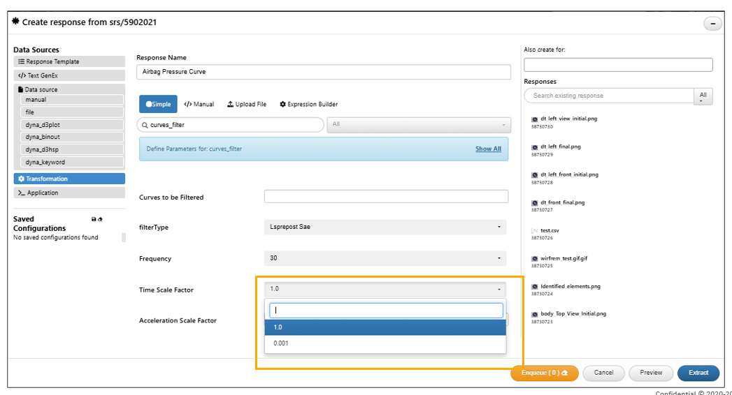
Scale factor options
This process is the same depending if you are comparing from the Physical Tests or Simulations page. To see how this is done via a step-by-step image explanation, please navigate to the Physical Tests section on Comparing Responses.
6.8. Extracting Responses
As mentioned earlier, create a new response by modifying simulation data under “Extract Response” in the Simulation Responses tab.
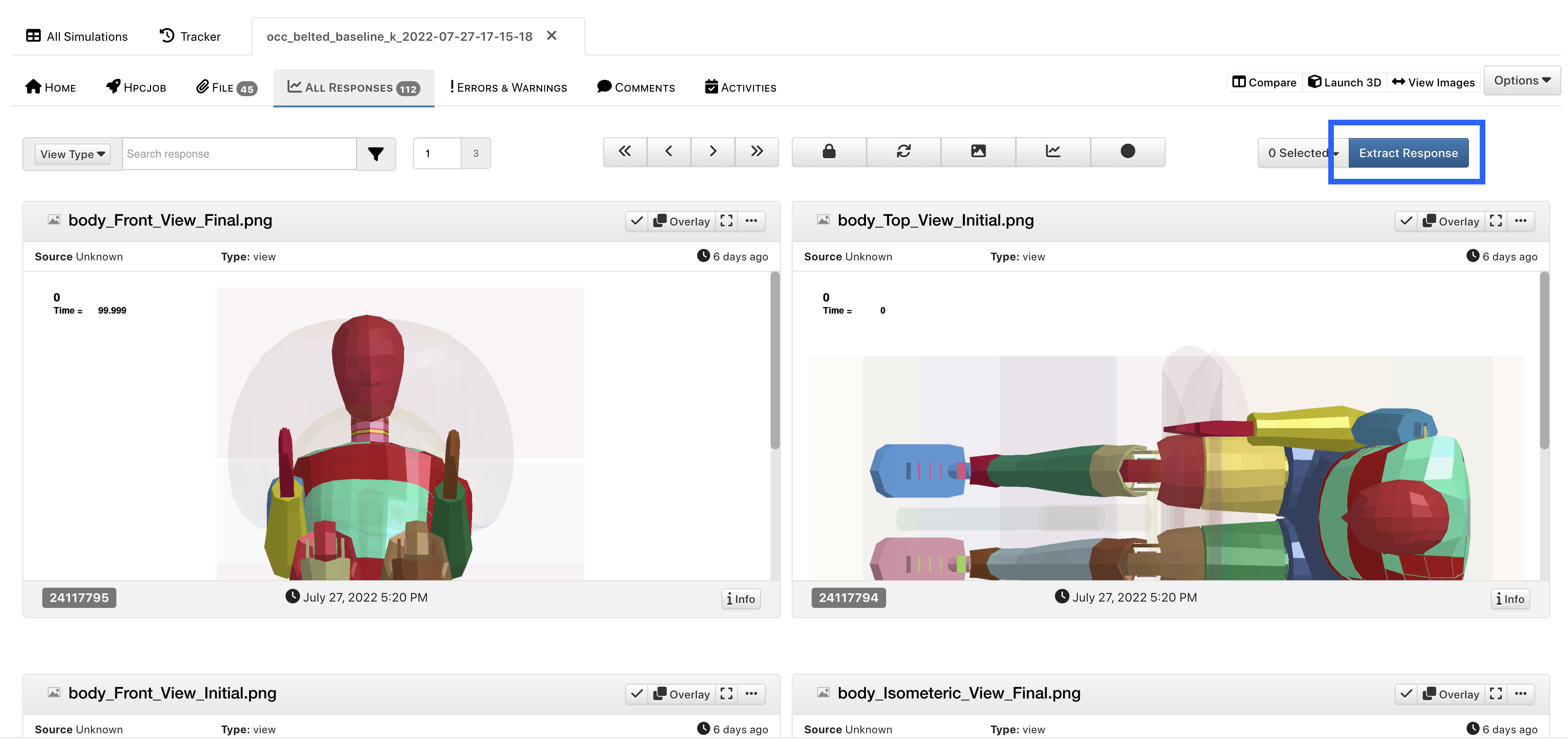
Figure 1: Choose Extract Response
In the next window, you can choose from a few different data extraction options. The most common ways to extract data will be from a data source (1) or employing a transformation (2). For data sources, available options will be dependent on the database files of the simulation.
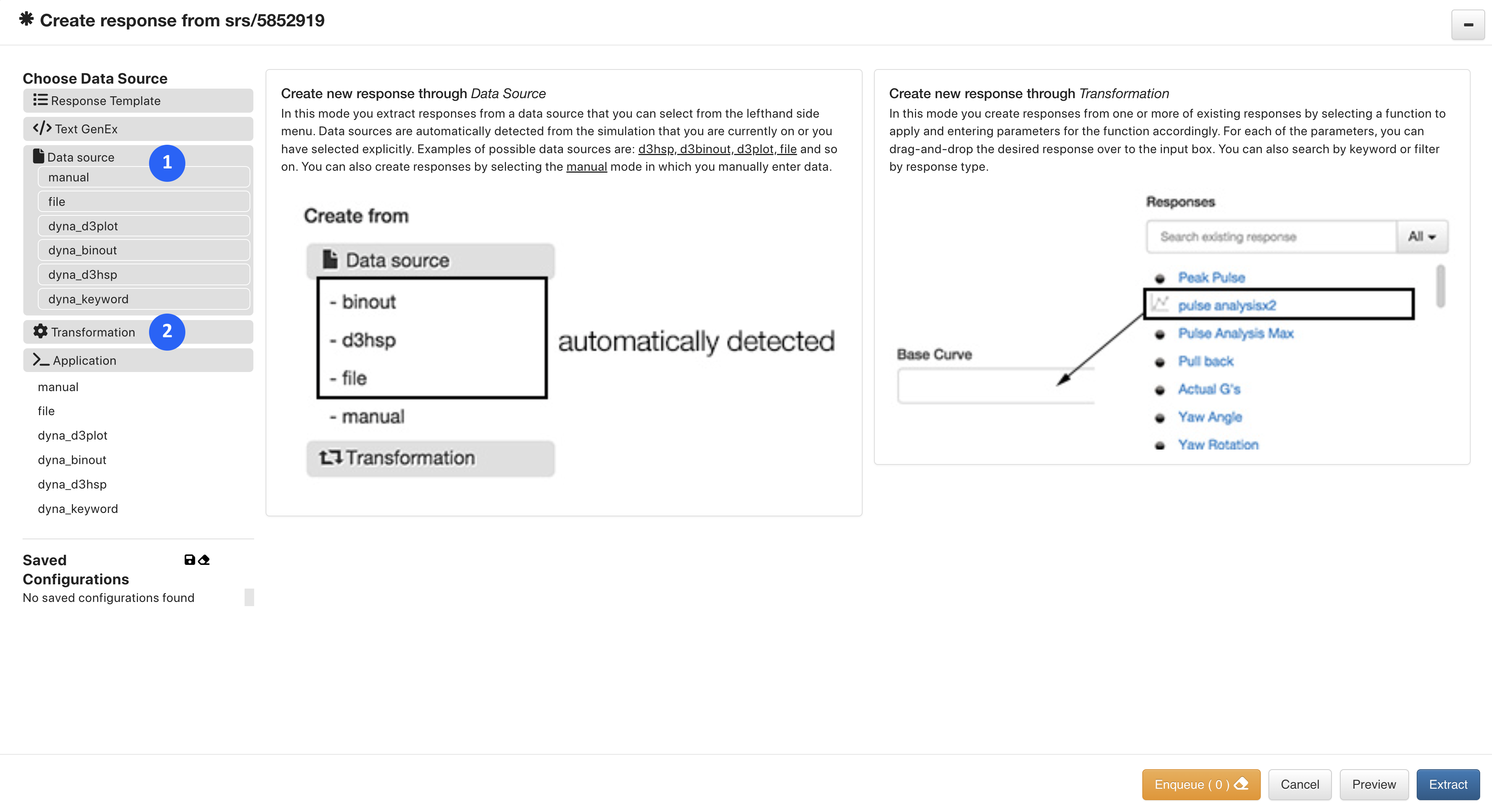
Figure 2: Choose Extraction Data Source
Finish all extractions by choosing “Extract” (1). Feel free to see a preview of your extraction first by clicking “Preview” (2).
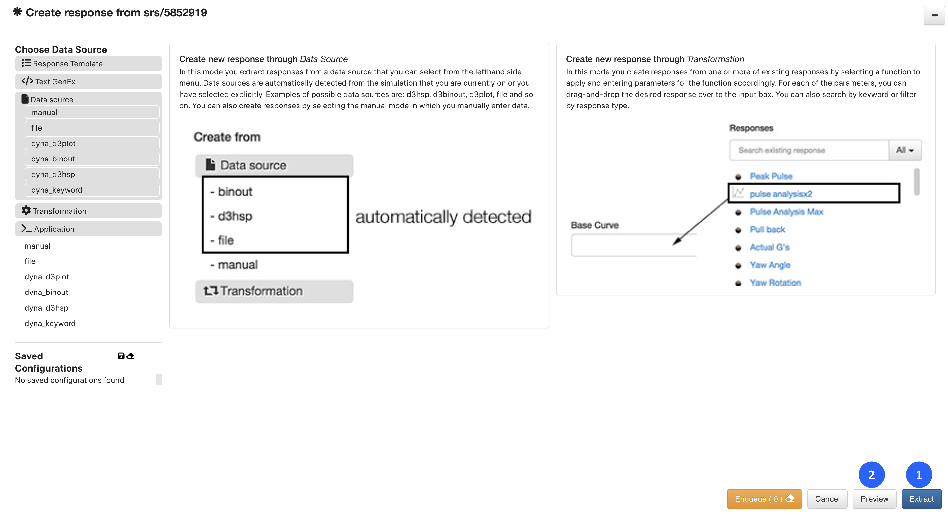
Figure 3: Finish Extraction
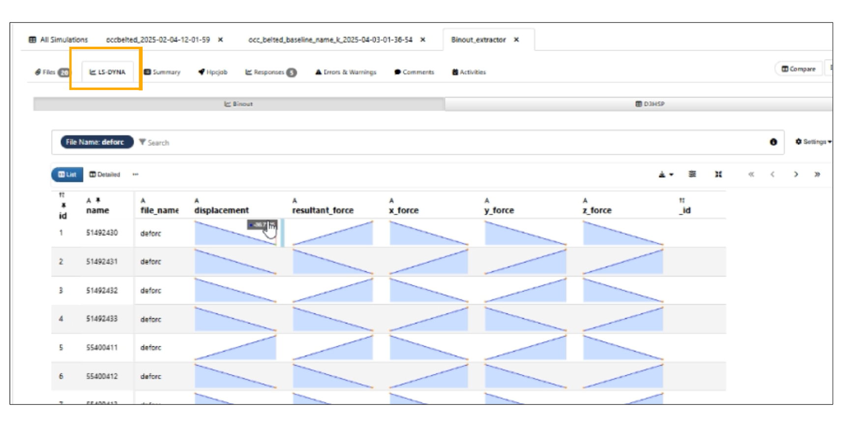
Binout Extractor
The ls-dyna binout (binary output) extractor post-processes a variety of simulation files efficiently. Depending on the type of simulation, we’ll have a list of different file types we can choose. Here are the options available for a Occupant Belted simulation:
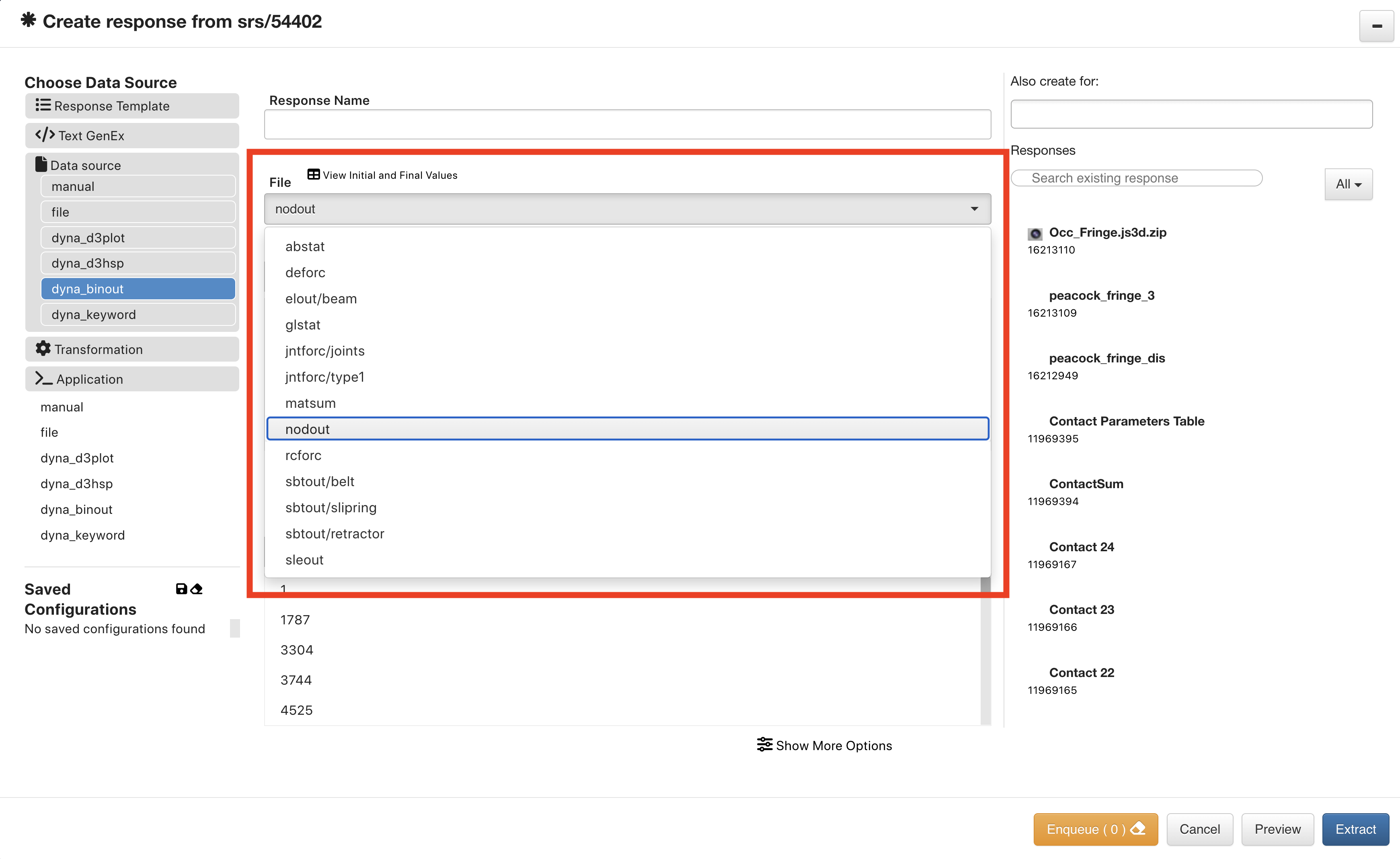
Figure 4: Binout Extractor Choose File
Here we’ve chosen nodout as our file type. The boxes show the labels and IDs of all database options available.
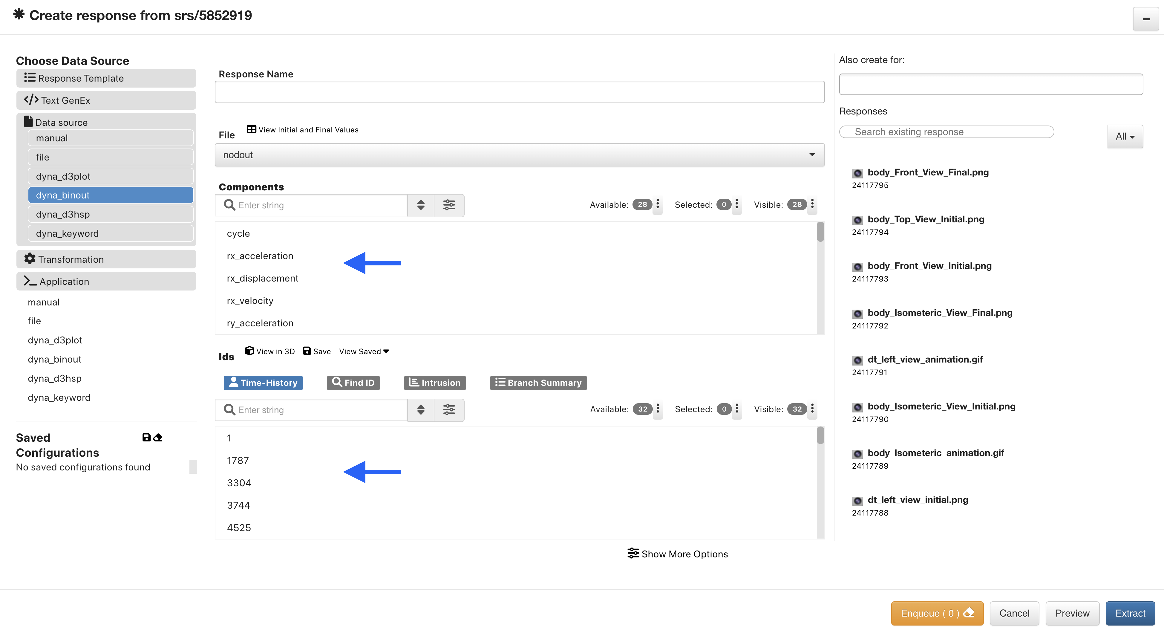
Figure 5: Binout Extractor
Then, we’ll select our components and IDs in the multi-select boxes. In this video example, we name our extraction “Displacement” and choose displacement components and node ID 1.
Binout Multi-Select
Find IDs
The Binout Extractor has an advanced feature for find specific IDs. We can use the Find IDs option instead of selecting IDs if we are unsure of which ID to select for a specific extraction. We’ll specify the scope to find a group of responses extracted as one and then decided which ID from the group we would like to extract individually. Let’s review an example using a Punch Specimen simulation.
After choosing binout in the response extraction window choose the file type (1), select the component (2) and name the response (3). Here, we are choosing elout/shell for the file, lower_eps_xy as the component and naming the response as such. We’ll then want to click on Find ID under the Ids section (4).
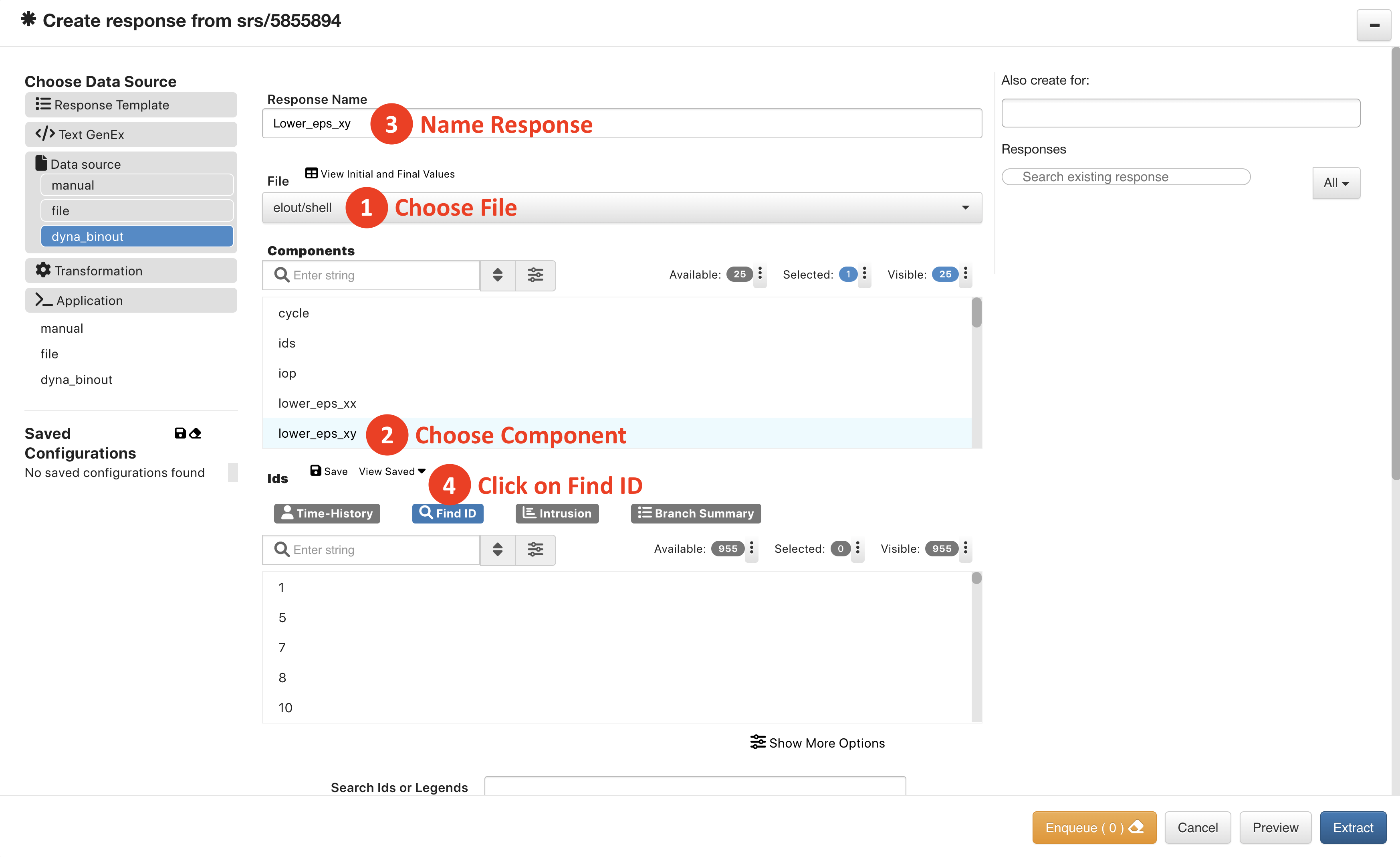
Figure 6: Choose File, Component and Find ID
This will give us a list of options we will fill-out as the scope for extracting the group of responses (scroll down to see them all). Here, we are choosing Any ID value (1), Any State (2), Sort by Y Max (3), Descending (4), and 5 as the Limit (5).
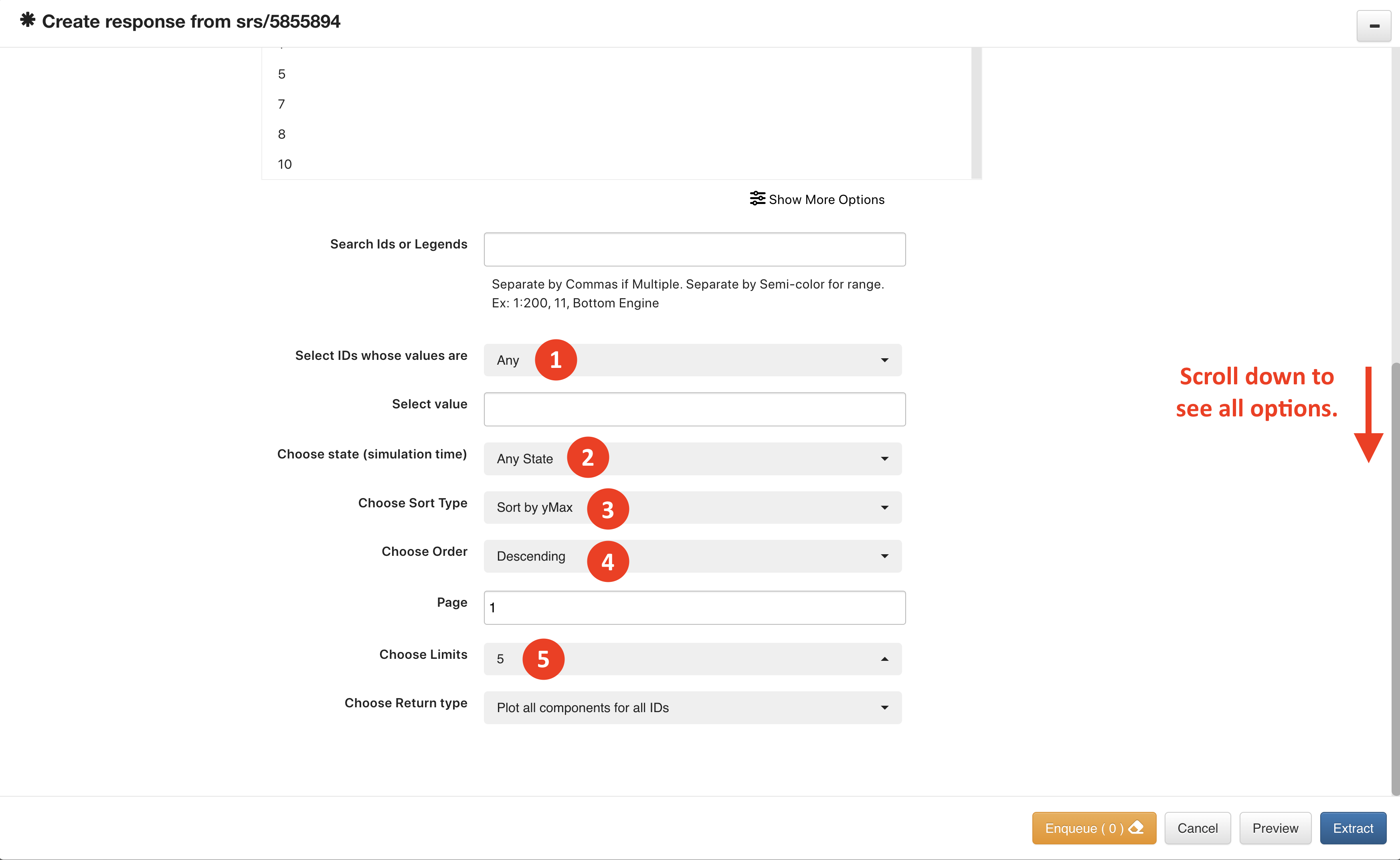
Figure 7: Find ID - Fill Out Scope
Click Extract to add the response. We’ll see (1) in the Enqueue as the extractor is processing.
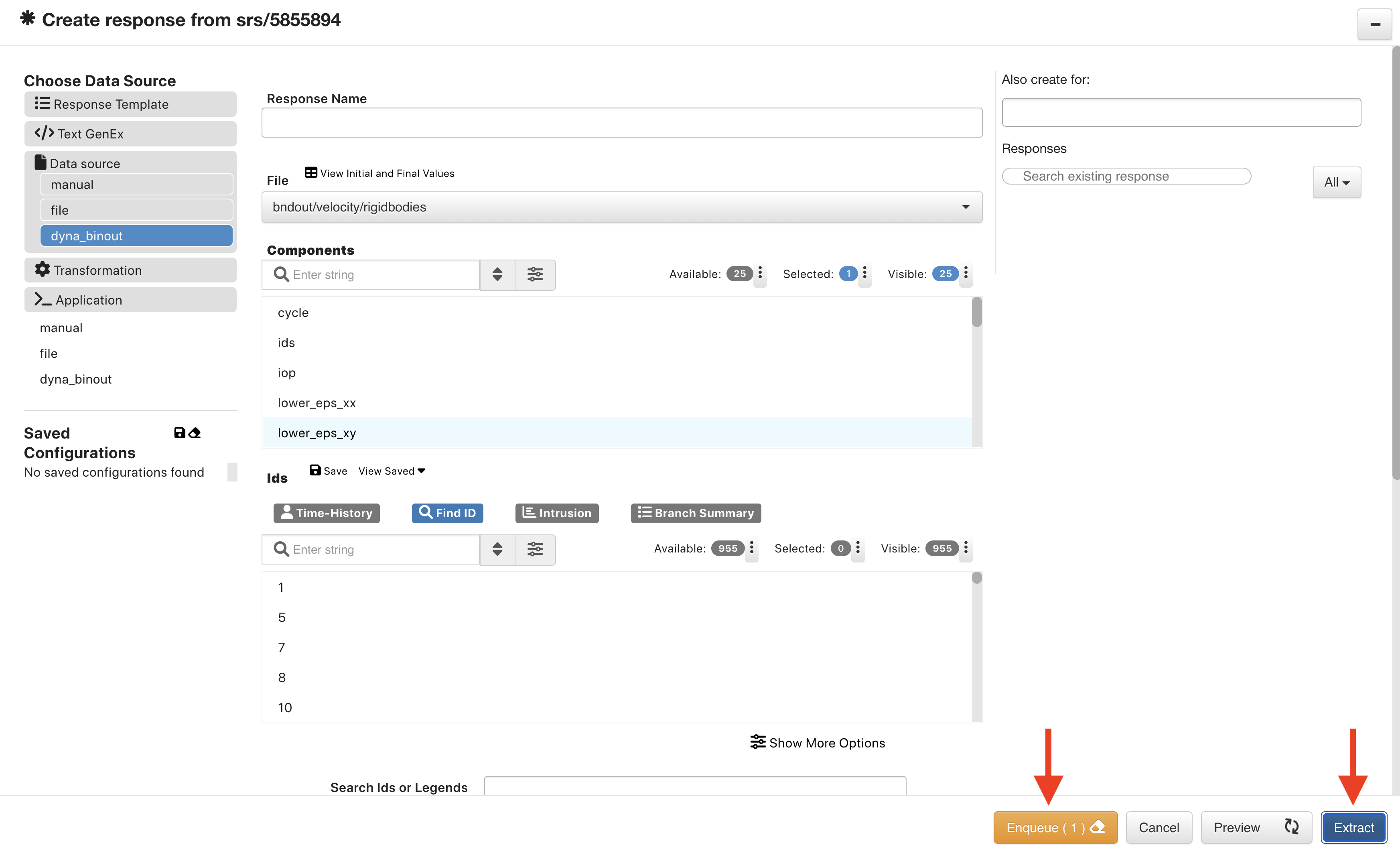
Figure 8: Extract Group
Under our simulation responses, we’ll see the newly extracted response group. For this Punch simulation, we have a group of curves and want to look for the ID of the curve with the highest peak: the blue curve with ID 439.
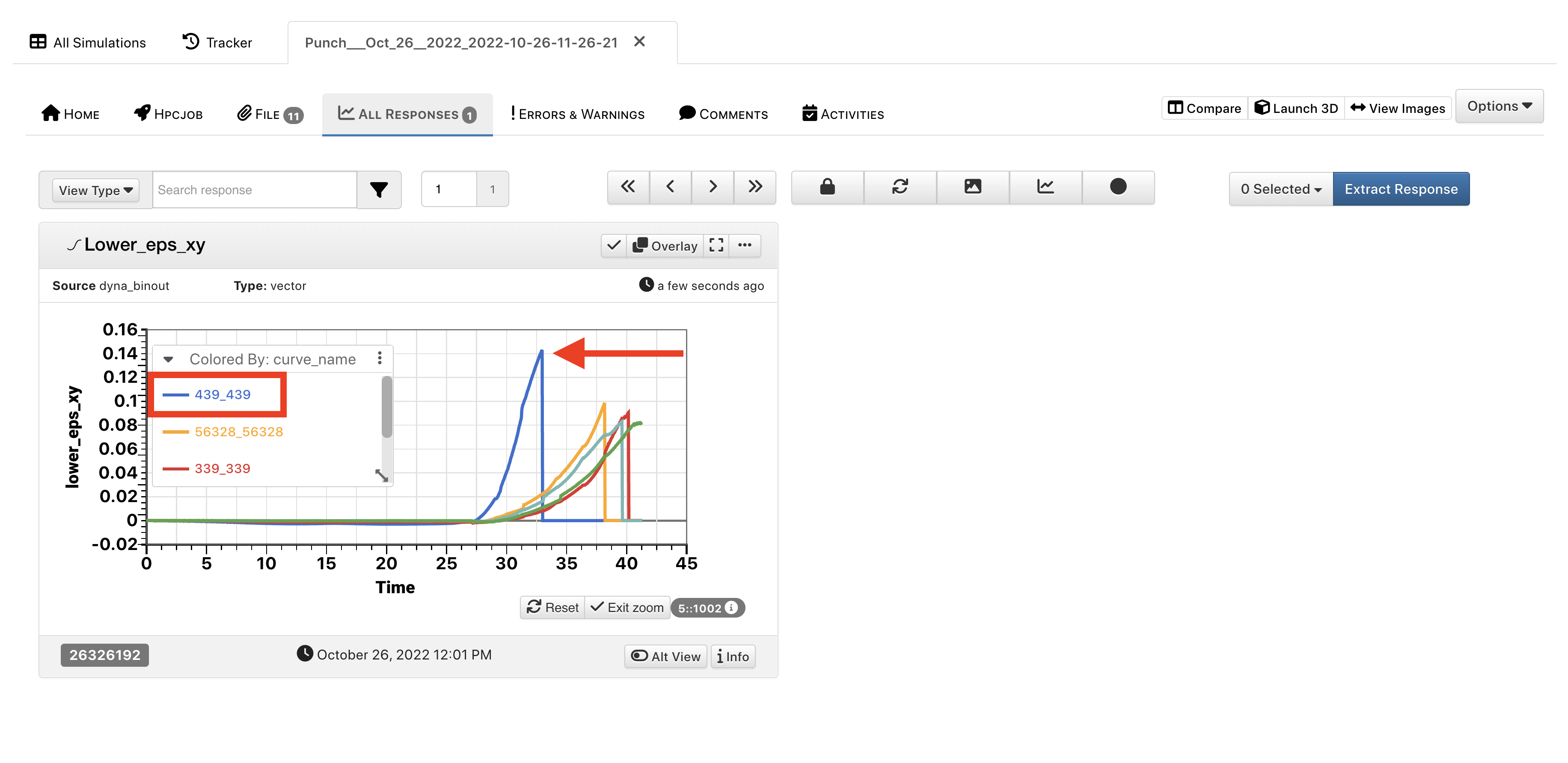
Figure 9: Find ID for Highest Peak
Now, we can go back to our binout extractor and just extract that curve. Here are the settings we’ve chosen for it. The same file and component, but now we are searching for the 439 ID and selecting it. Make sure to give this response a unique name.
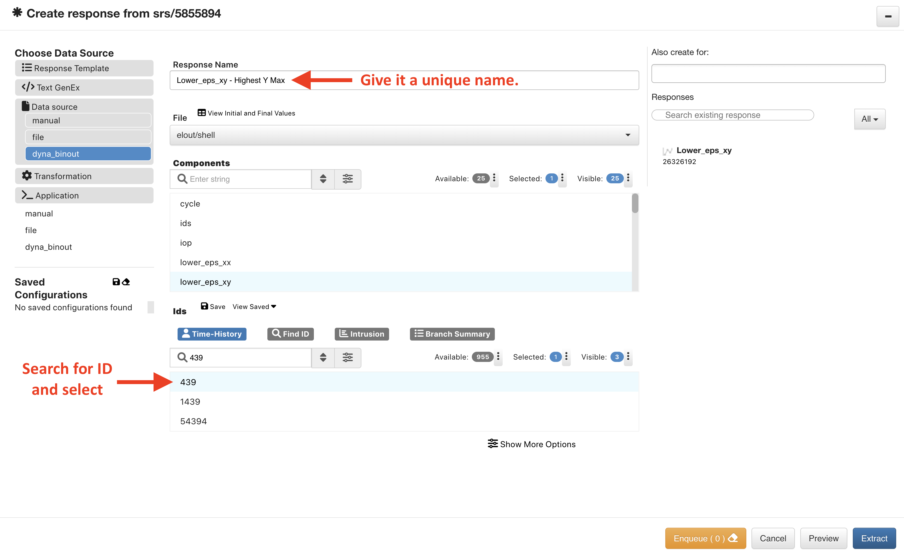
Figure 10: Extract Highest Peak
Once we extract, we’ll see the curve with the highest peak as an individual response in our simulation.
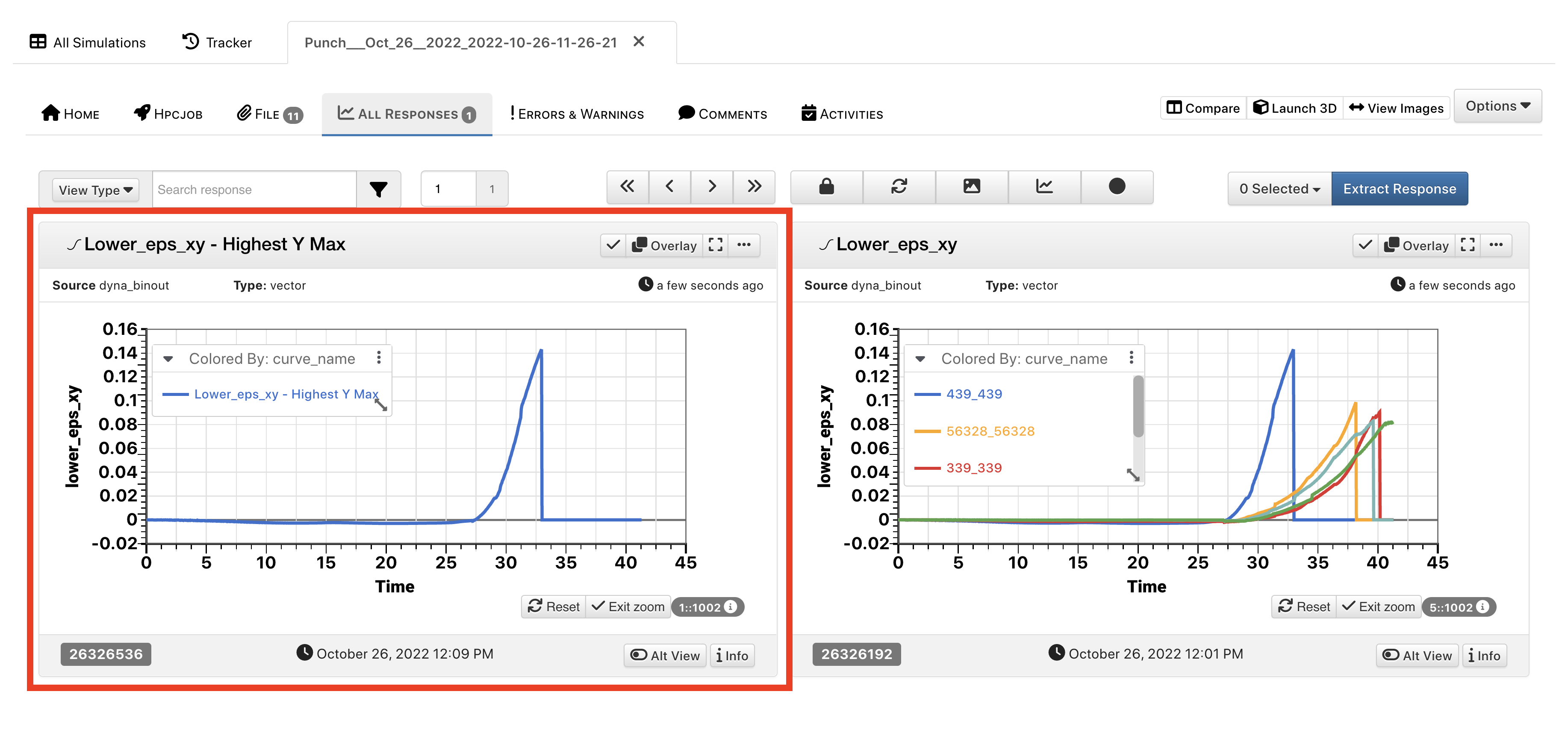
Figure 11: Highest Peak Response
Binout responses can be extracted for the elout/shell files in the Simulations.
SSSTAT files
In Simulations, SSSTAT files now allow access to mass and mass center while extracting binout responses.
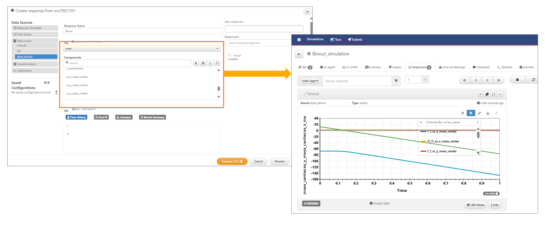
SSSTAT files
d3plot Extractor
The ls-dyna d3plot extractor post-processes simulations in 3D visualizations and animations. d3plot is most commonly used for creating 3D models (with or without plastic strain) of our simulations but has an array of file options.
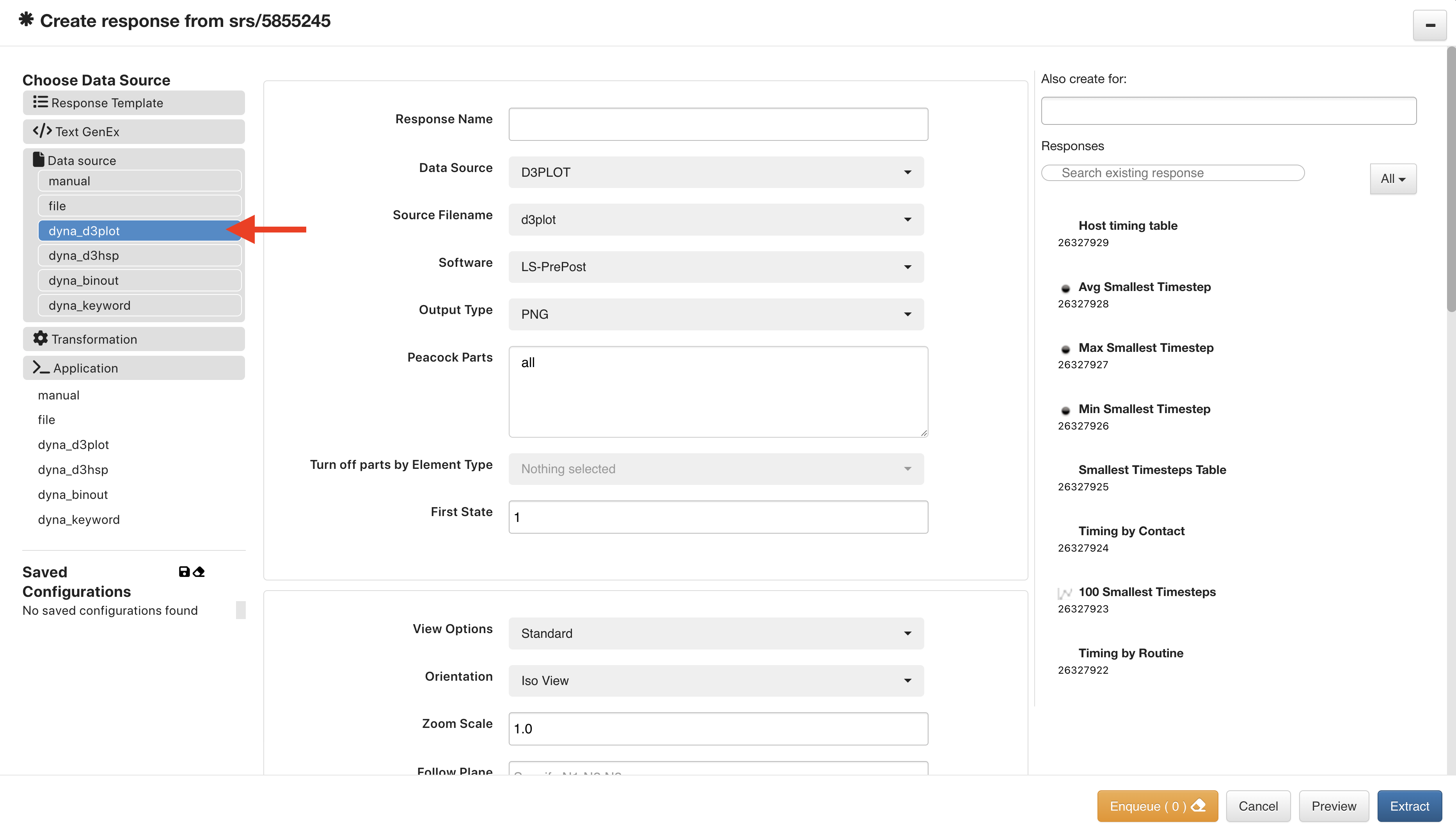
Figure 12: d3plot Extractor
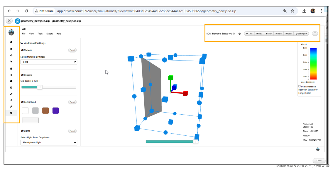
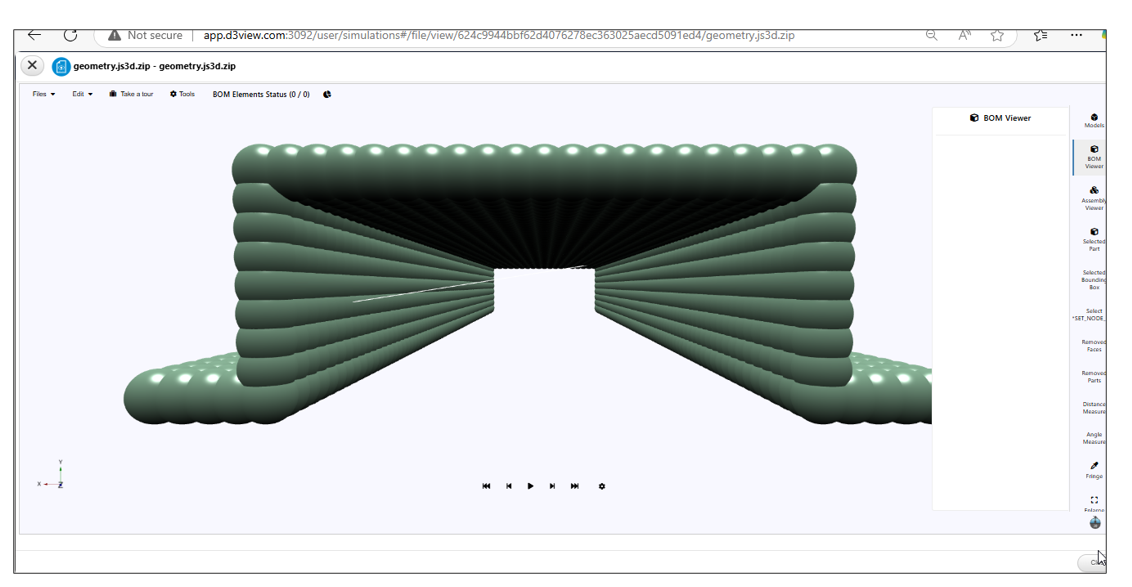
Let’s review how to create a Peacock model using d3plot extractor. First, we’ll name out response and make sure to end it with the js3d.zip file extension for viewing in Peacock (1). Then, we’ll choose Peacock3D as our output type (2). Next, we’ll choose the Plastic Strain fringe type (3). (There are also options for von-Mises Stress and Thickness). Lastly, we’ll indicate the final state to be 100 (4). All other options can remain as the default (or as shown in the following image). Click extract to finish.
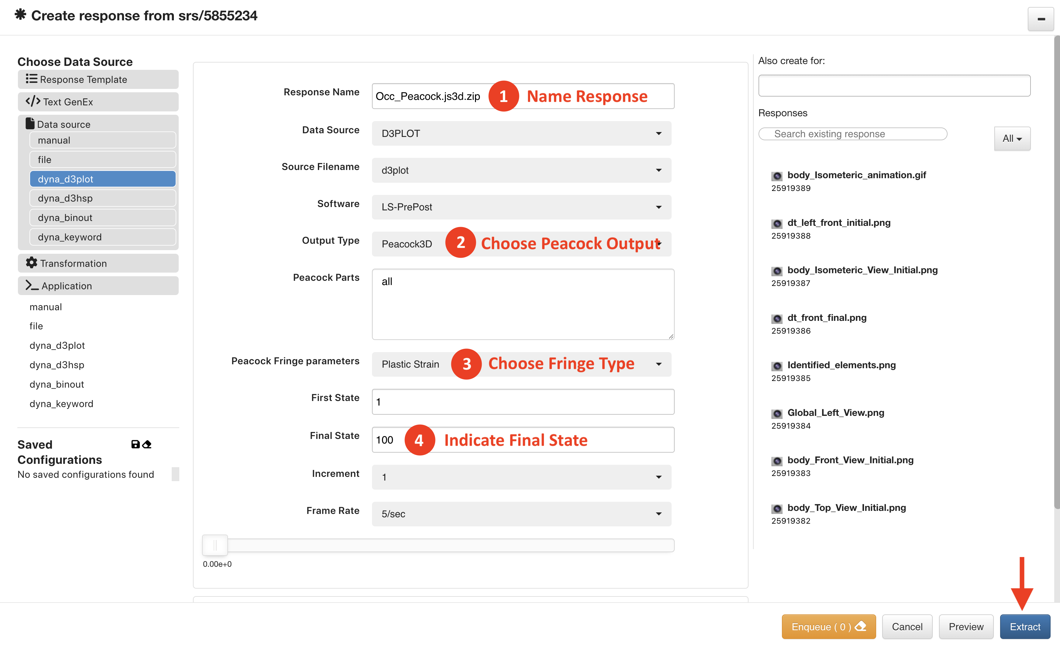
Figure 13: d3plot Peacock 3D Response Set-up
On our simulation responses tab, we’ll see our new response with a Peacock logo. Click on the logo to initiate it in peacock.
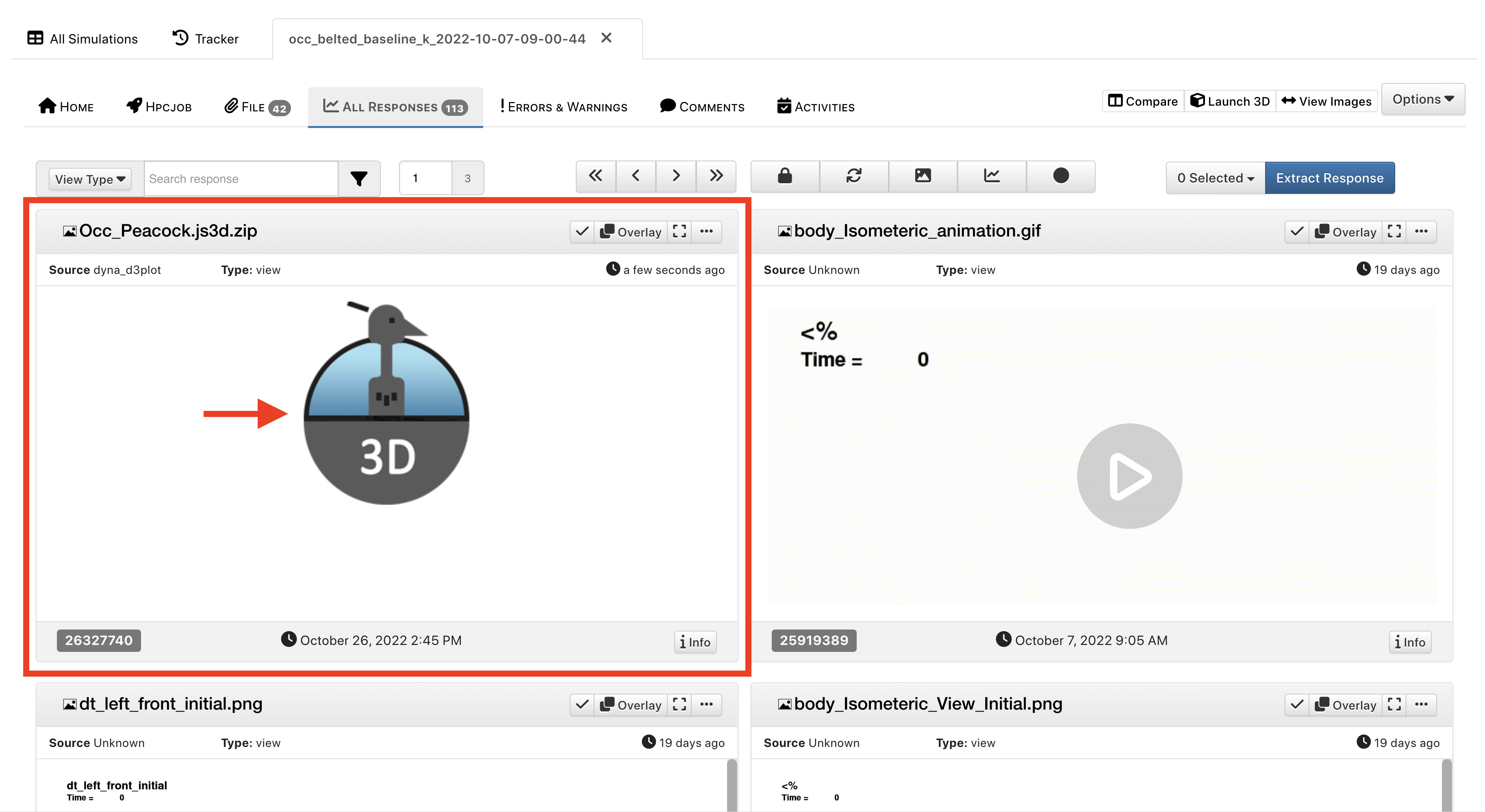
Figure 14: Peacock 3D Response in Simulation
We can now explore the model in 3D space. To learn how to navigate Peacock, check out that section here.
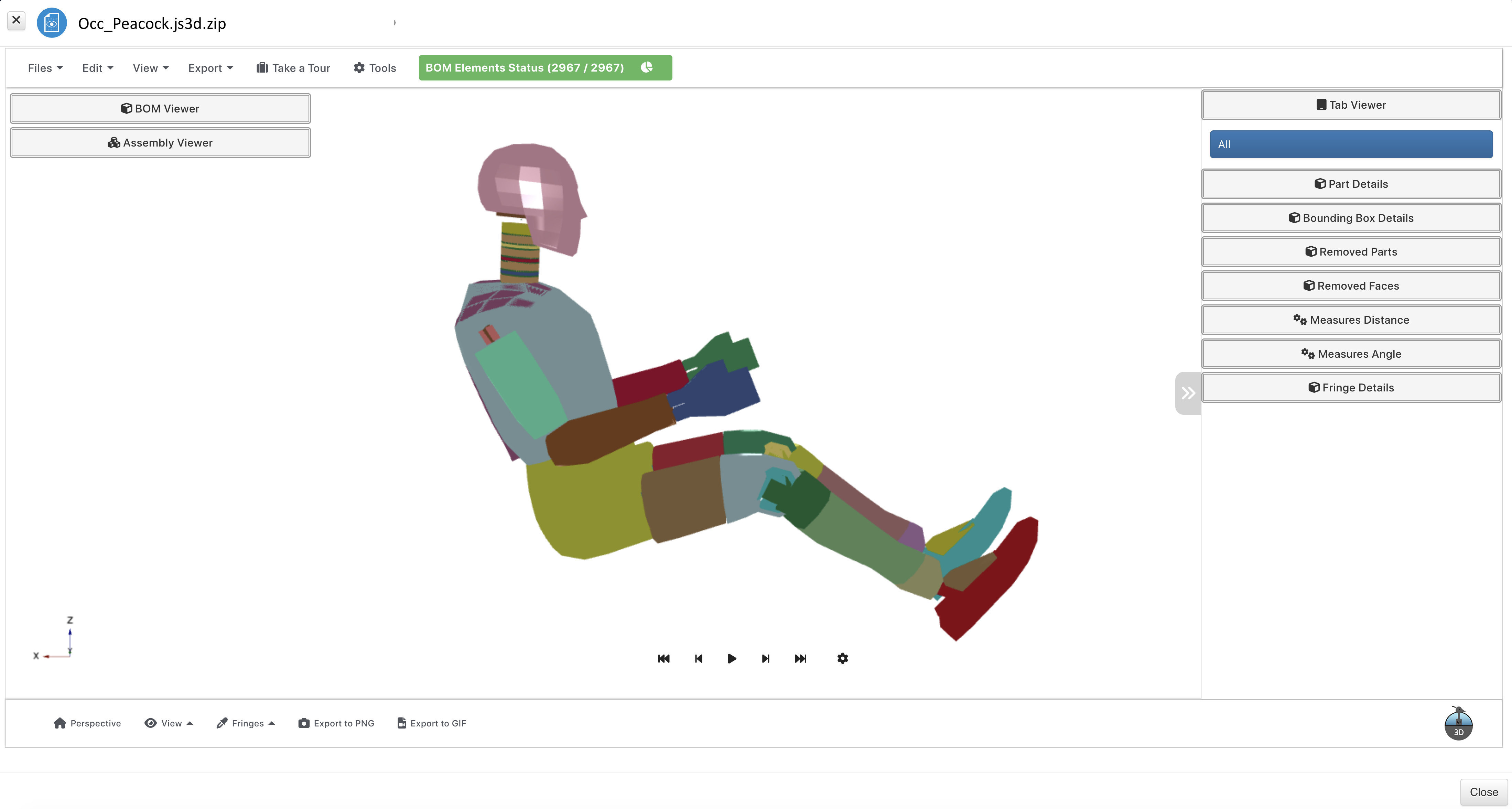
Figure 15: Peacock 3D Model
d3hsp Extractor
The ls-dyna d3hsp extractor is most commonly used to check the model information such as to investigate the causes of the simulation’s error termination, similar to a solver log. d3hsp can print all the information related the model and the solver states as the simulation is being solved.
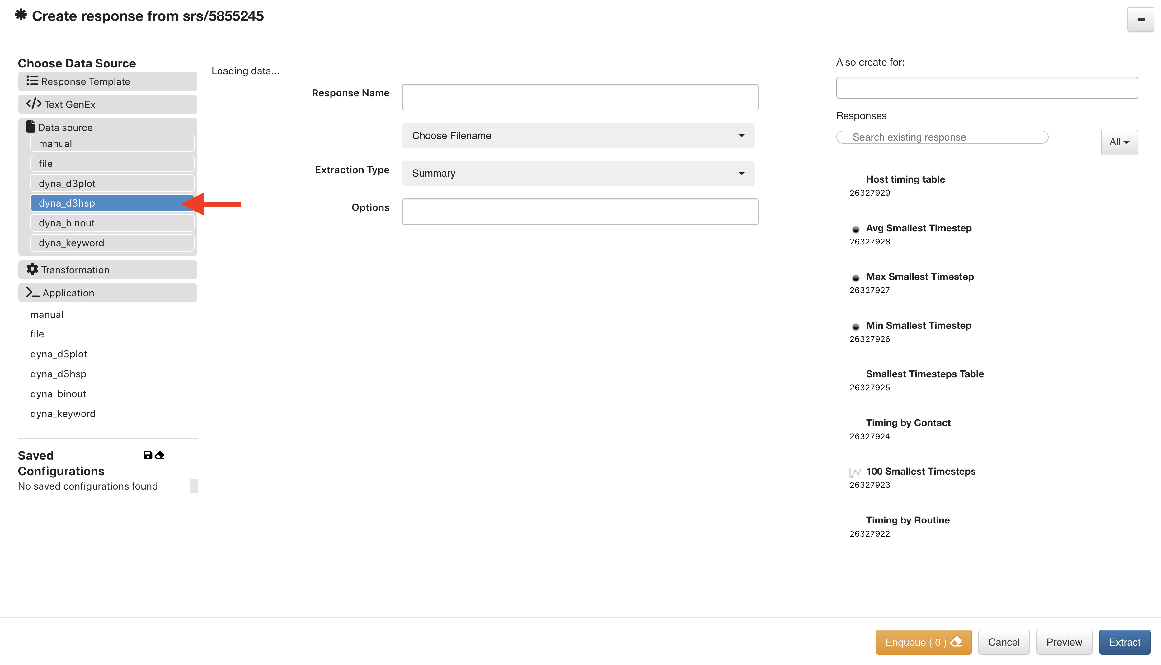
Figure 16: d3hsp Extractor
Here are all the d3hsp options available for extraction. Read on to see examples of each.
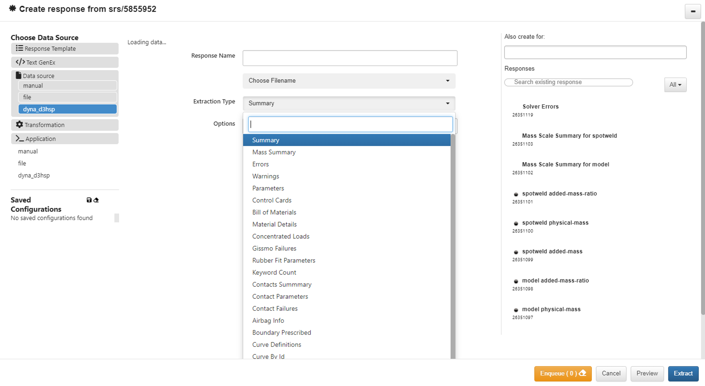
Figure 17: d3hsp Options
Mass Summary
For this set-up, we’ve chosen d3hsp for the file name, Mass Summary for the file type and named the response.
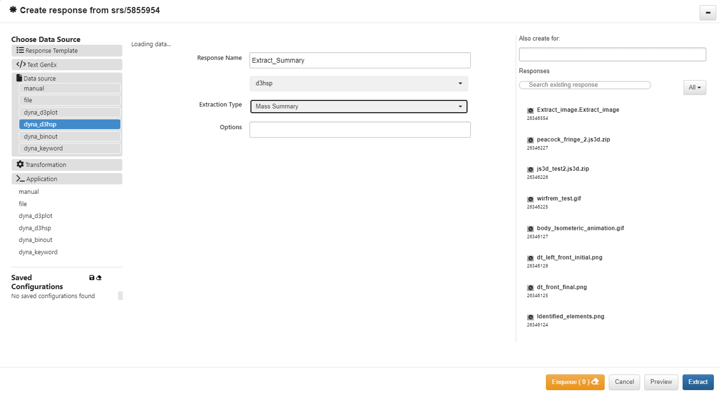
Figure 18: d3hsp Mass Summary
This extraction gives us individual summary responses for each aspect of the simulation execution.
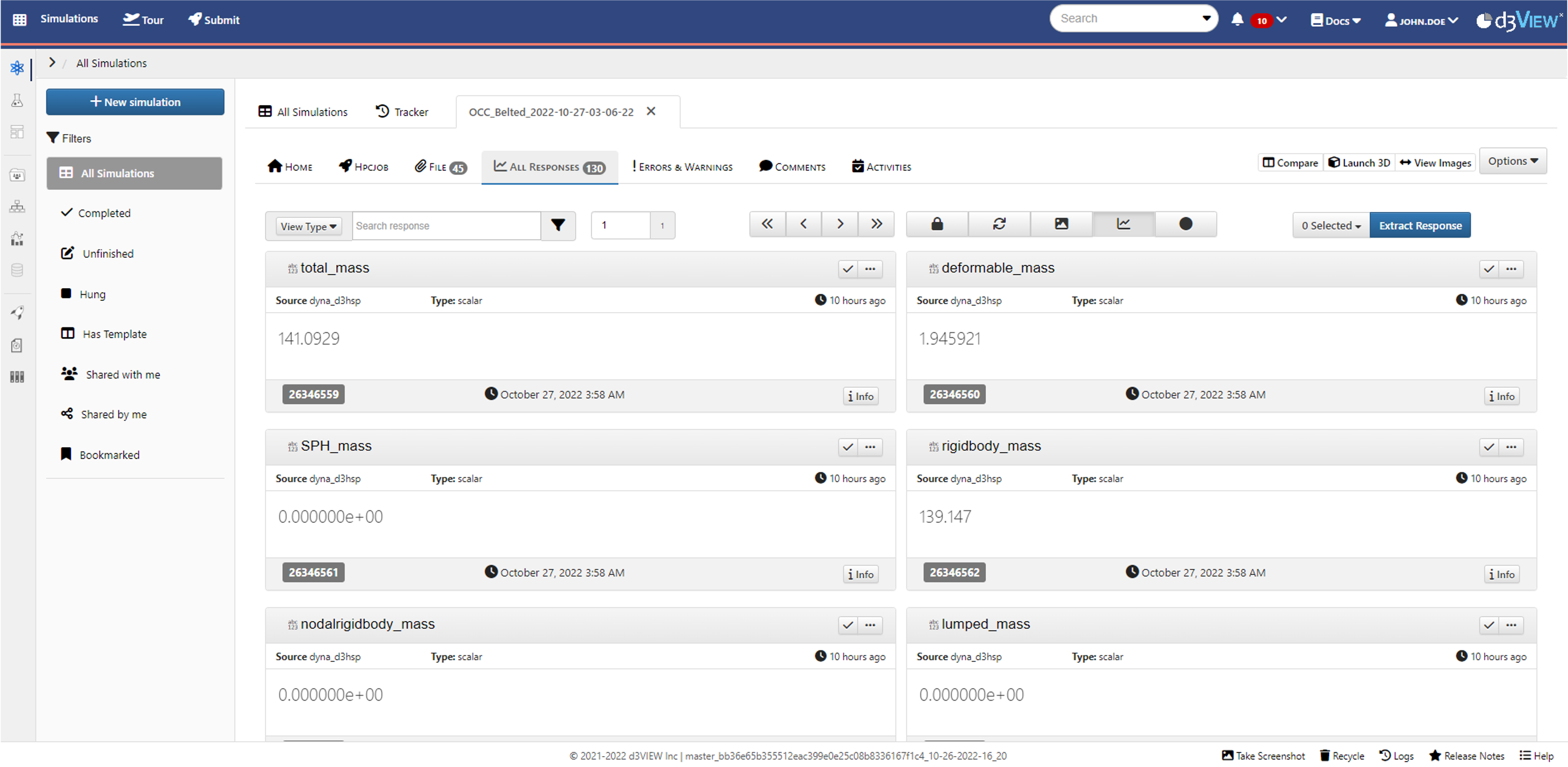
Figure 19: d3hsp Mass Summary Responses
Summary
For this set-up, we’ve chosen d3hsp for the file name, Summary for the file type and named the response.
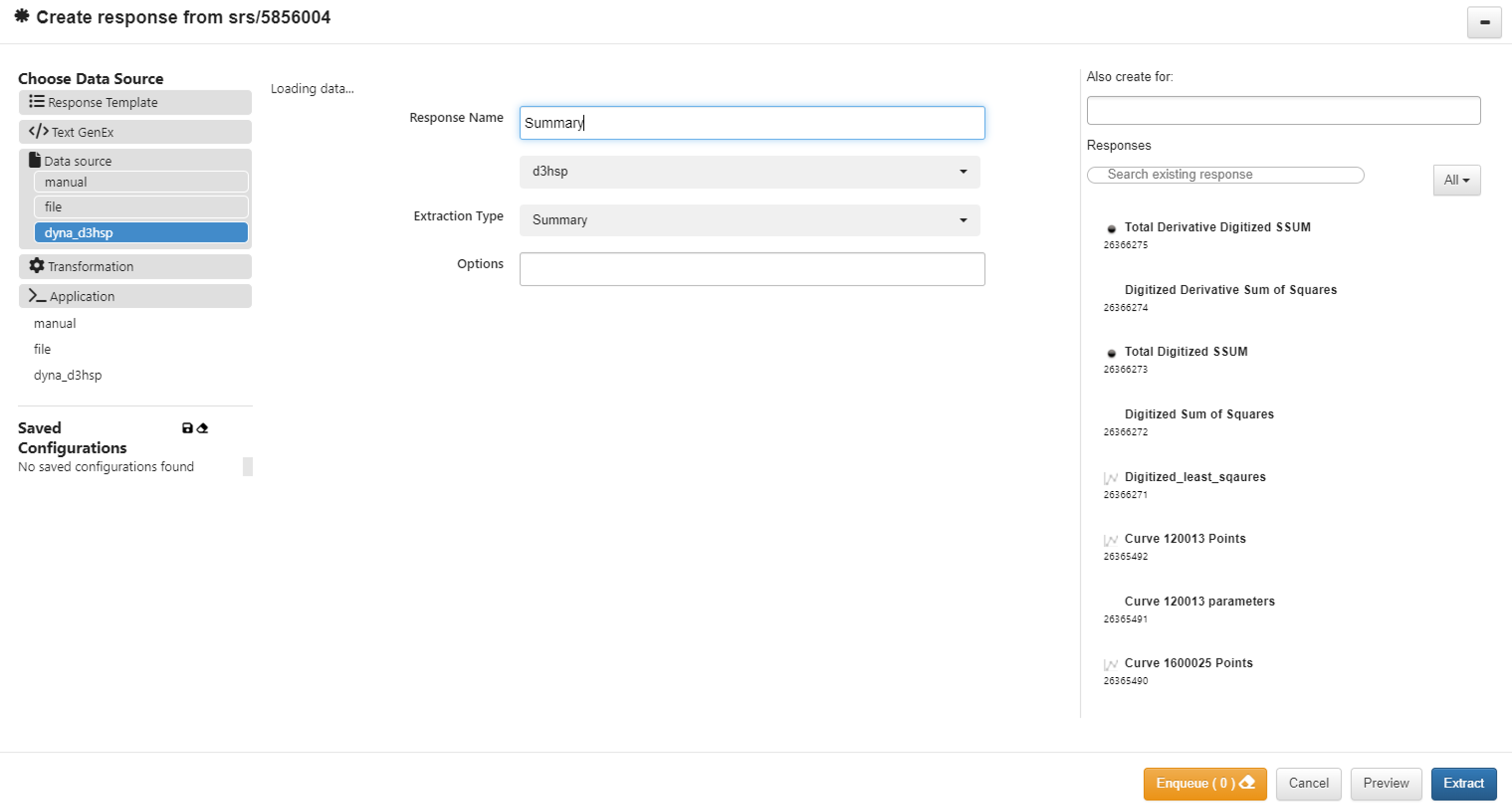
Figure 20: d3hsp Summary
This extraction gives us individual responses for a summary of the simulation execution.
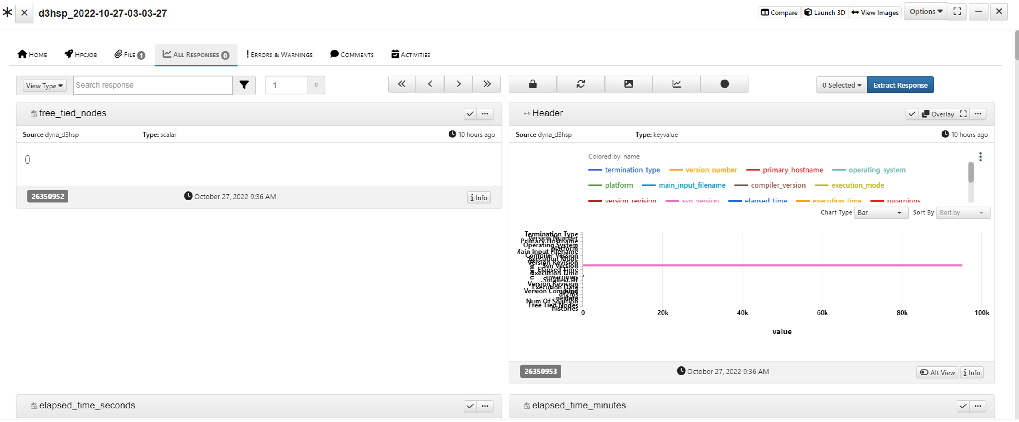
Figure 21: d3hsp Summary Responses
Errors
For this set-up, we’ve chosen d3hsp for the file name, Errors for the file type and named the response.
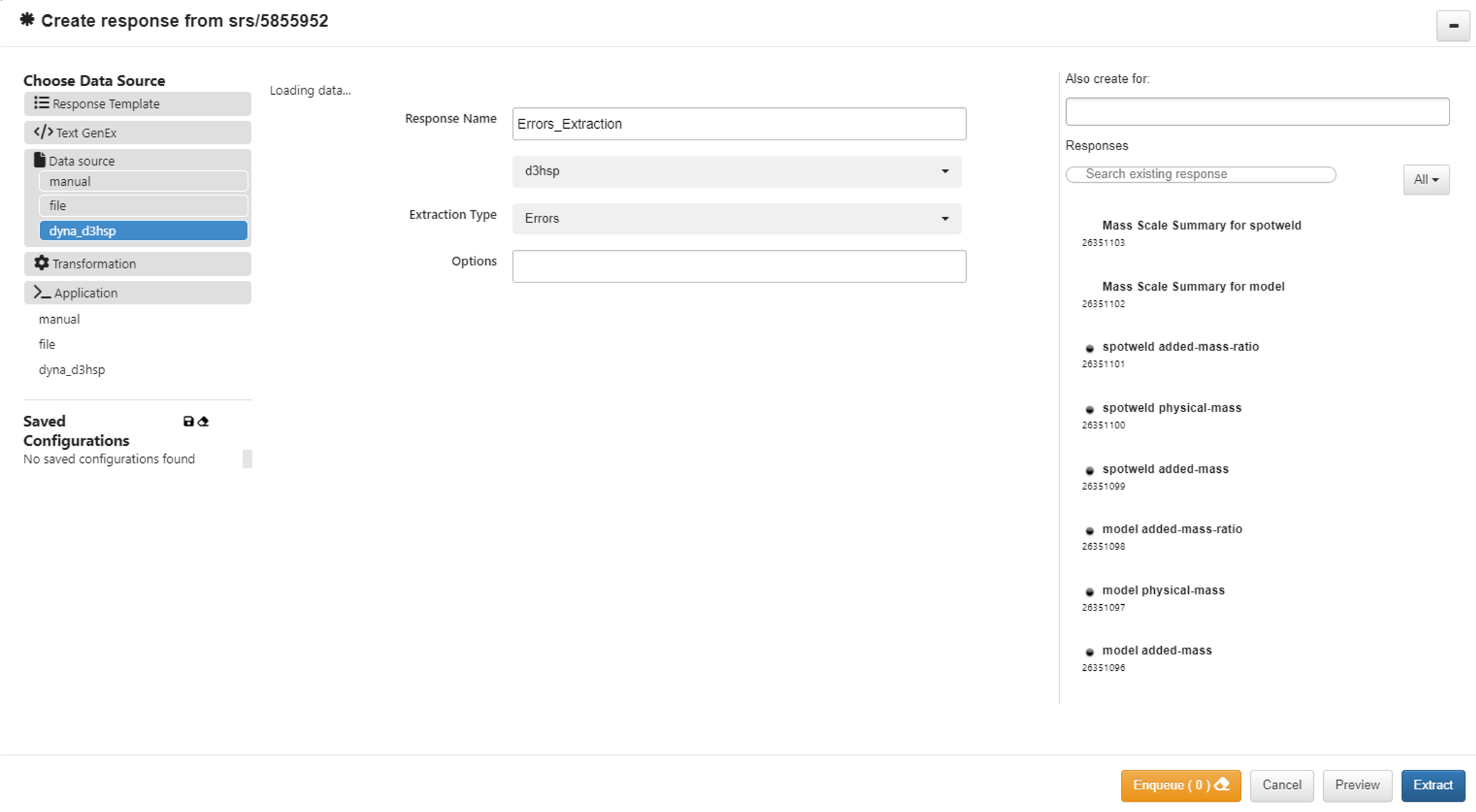
Figure 22: d3hsp Errors
This extraction gives us an individual response for solver errors.
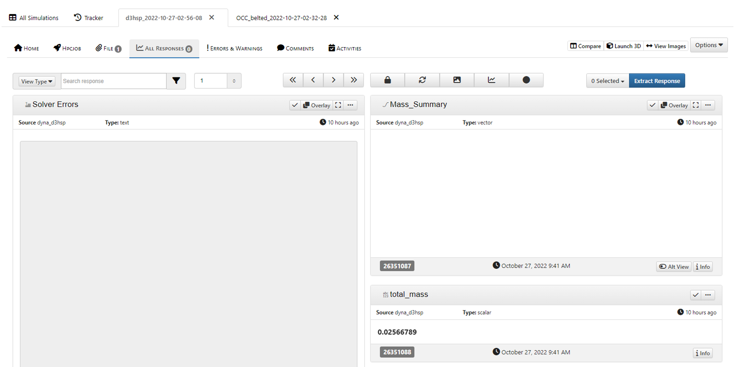
Figure 23: d3hsp Errors Responses
Warnings
For this set-up, we’ve chosen d3hsp for the file name, Warnings for the file type and named the response.
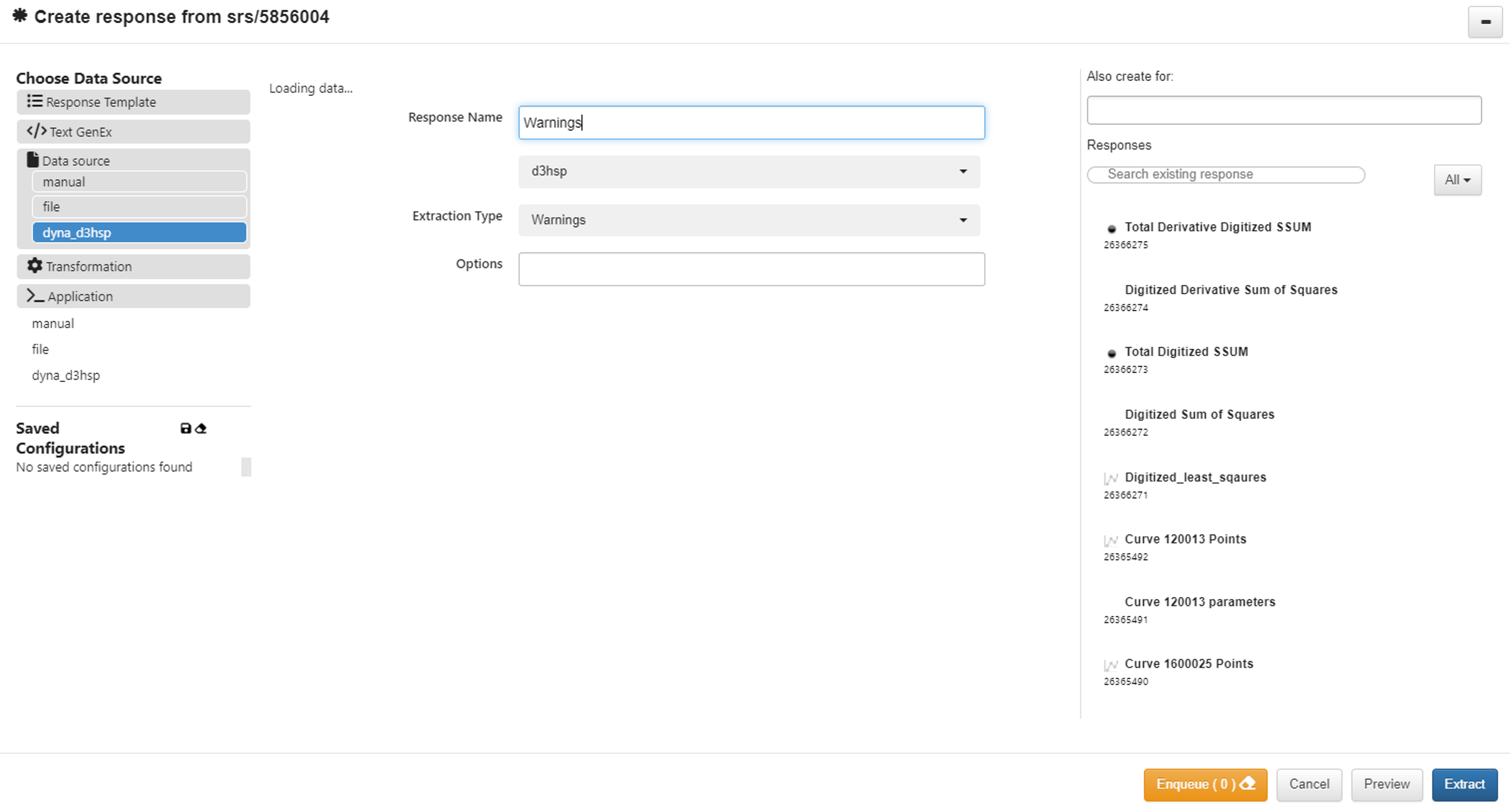
Figure 24: d3hsp Warnings
This extraction gives us an individual response for solver Warnings.
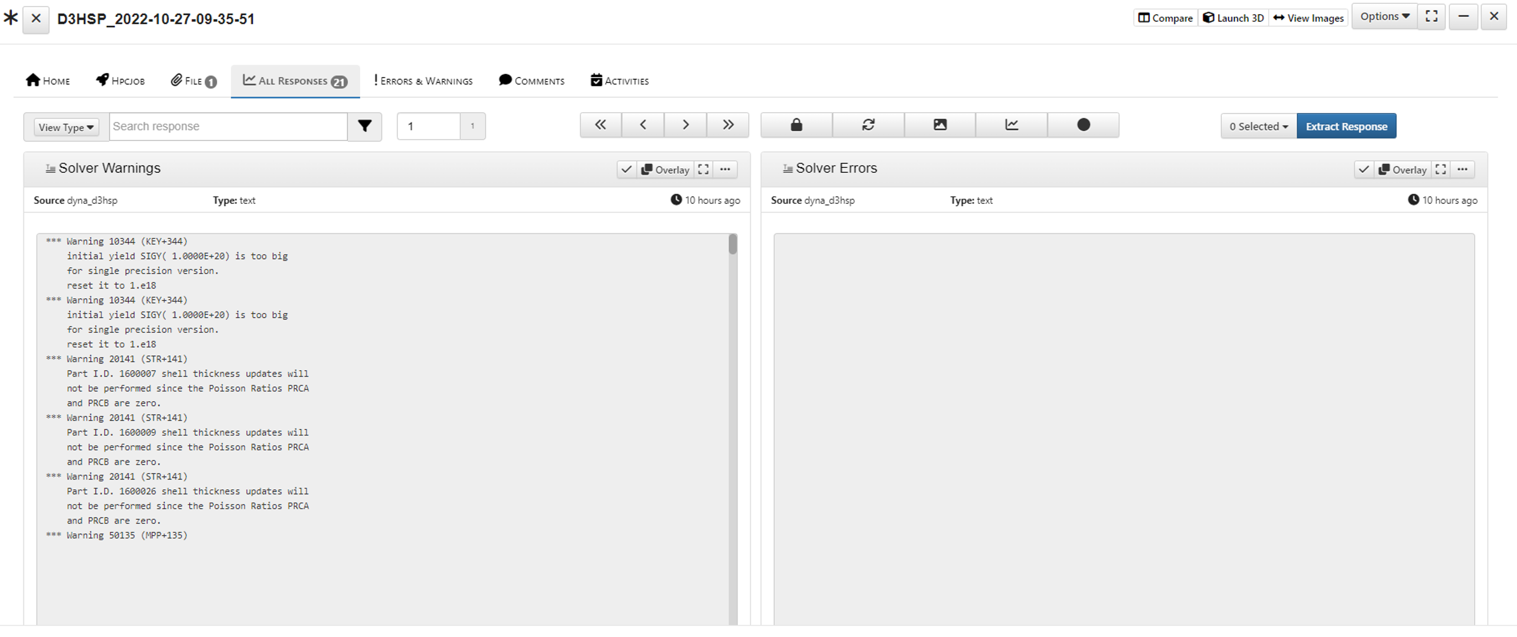
Figure 25: d3hsp Warnings Responses
Control Cards
For this set-up, we’ve chosen d3hsp for the file name, Control Cards for the file type and named the response.
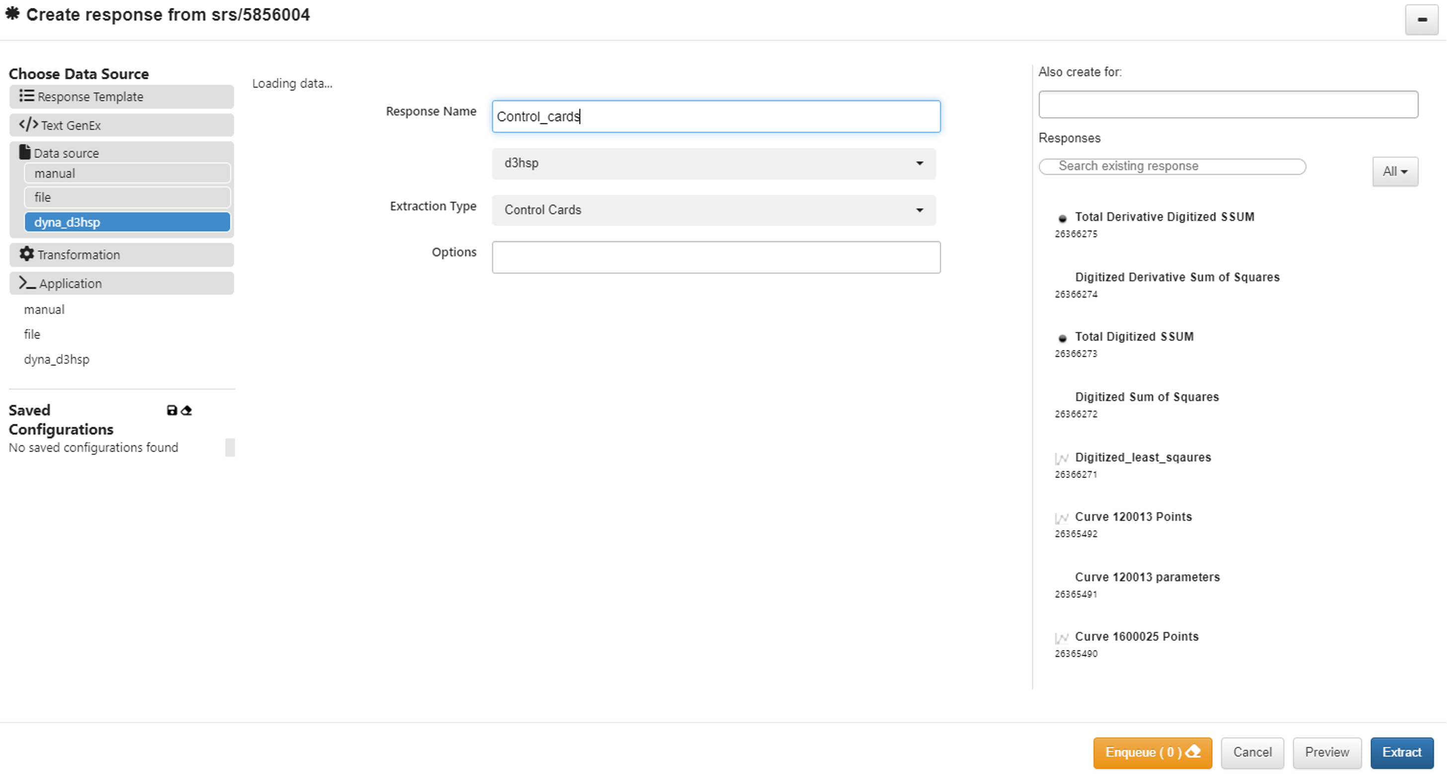
Figure 26: d3hsp Control Cards
This extraction gives us individuals responses for Control Cards.
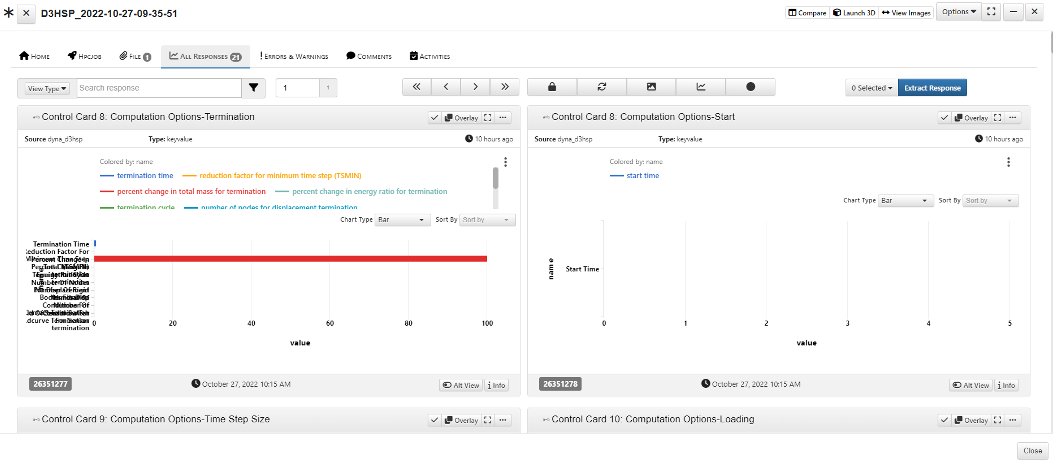
Figure 27: d3hsp Control Cards Responses
Bill of Materials
For this set-up, we’ve chosen d3hsp for the file name, Control Cards for the file type and named the response.
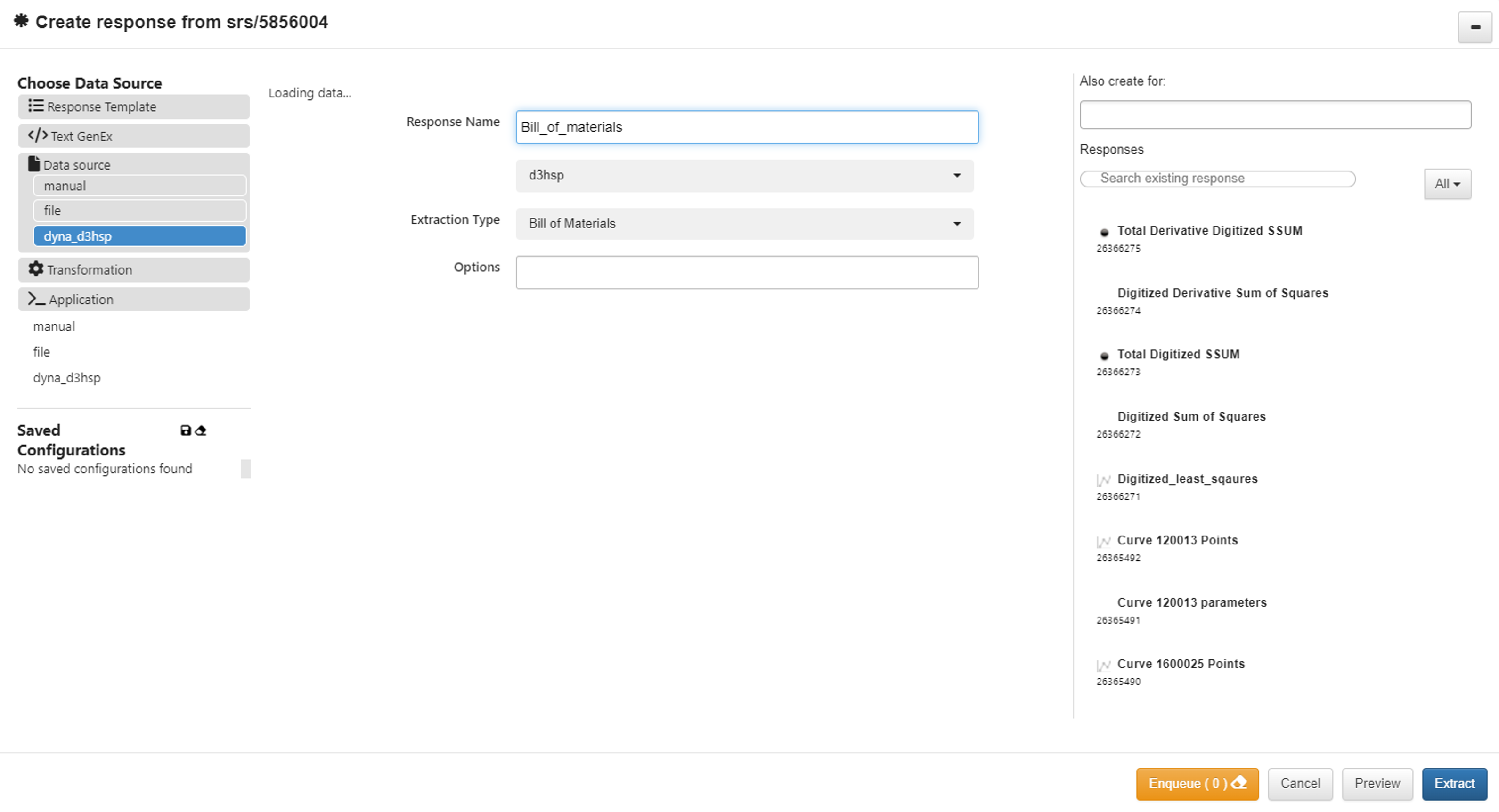
Figure 28: d3hsp Bill of Materials
This extraction gives us individuals responses for Bill of Materials.
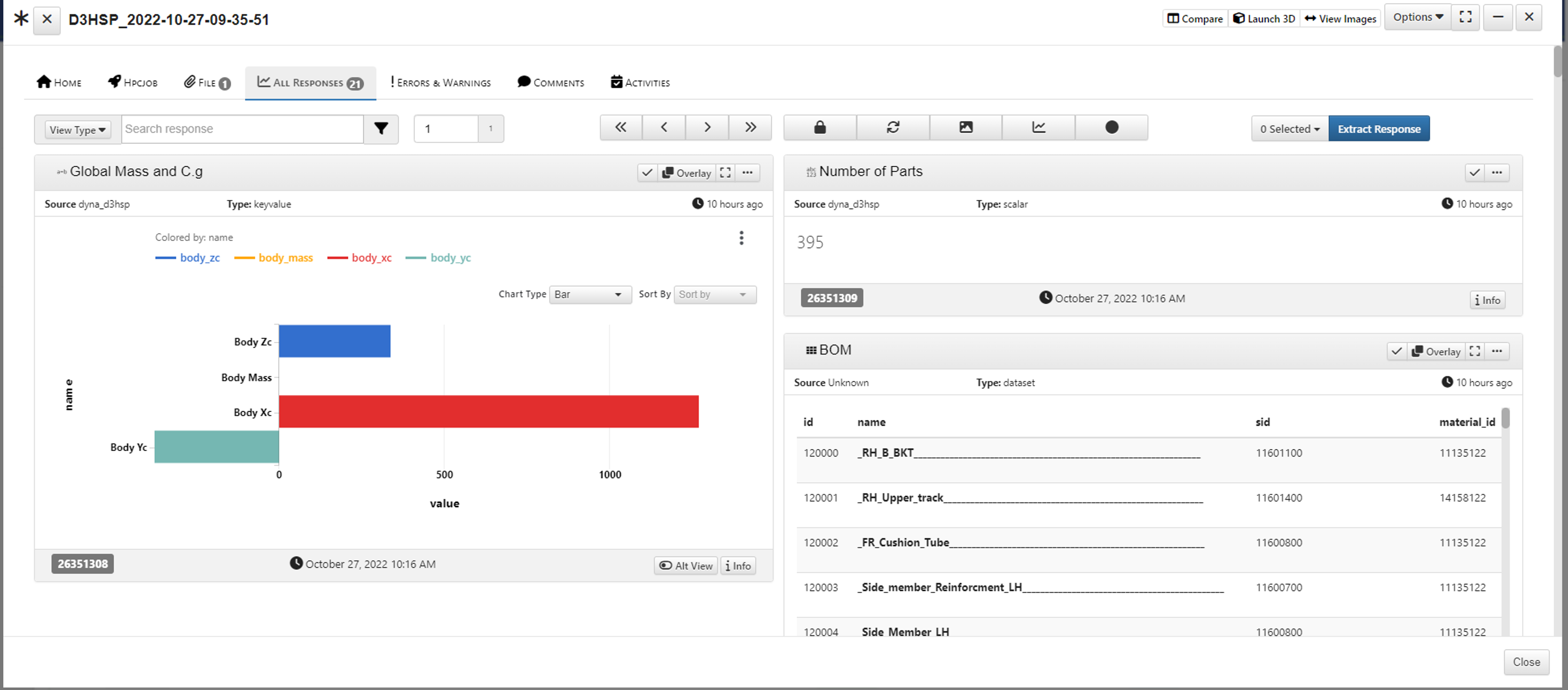
Figure 29: d3hsp Bill of Materials Responses
Material Details
For this set-up, we’ve chosen d3hsp for the file name, Control Cards for the file type and named the response.
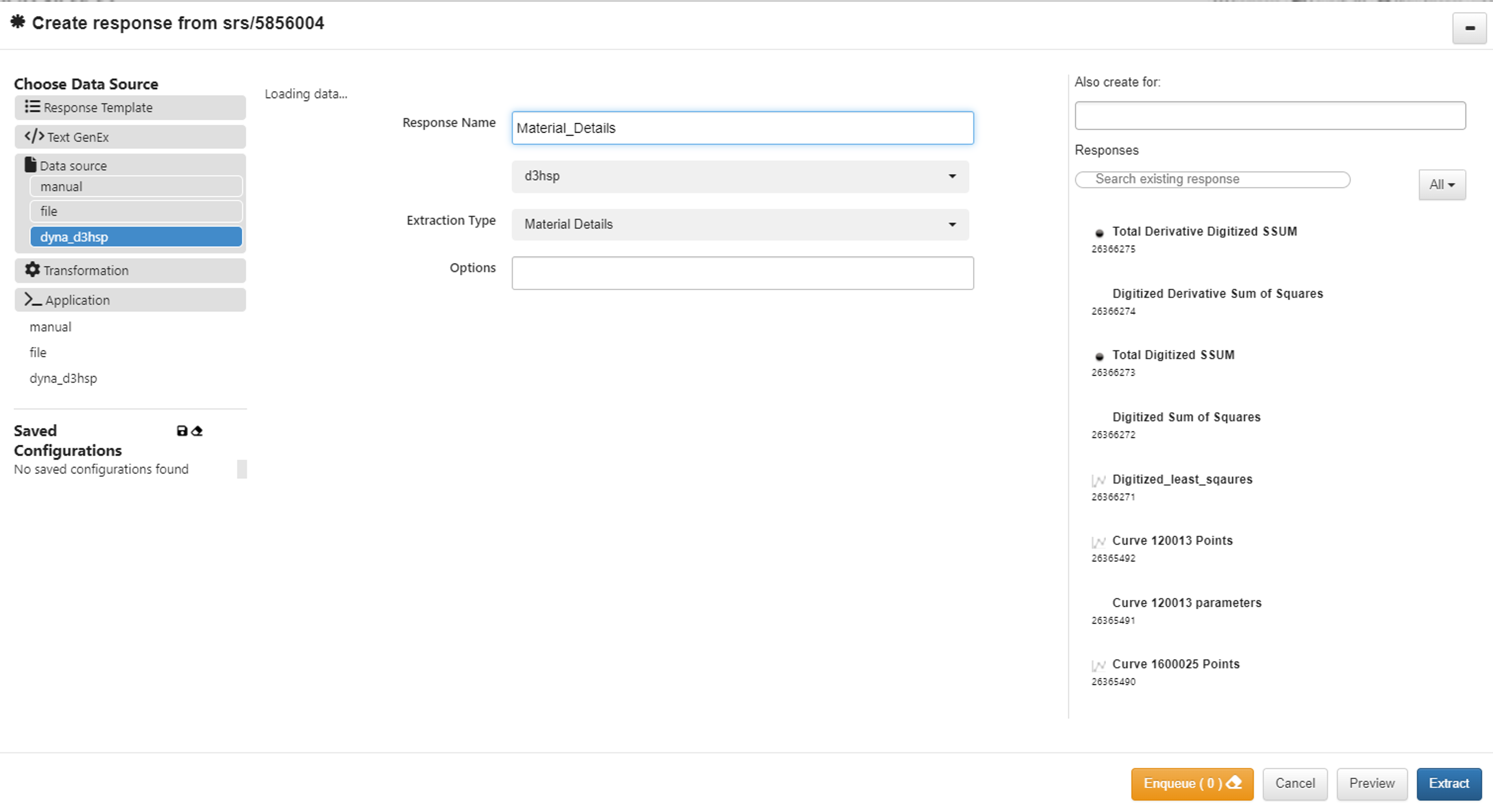
Figure 30: d3hsp Material Details
This extraction gives us an individual response table for Material Details.
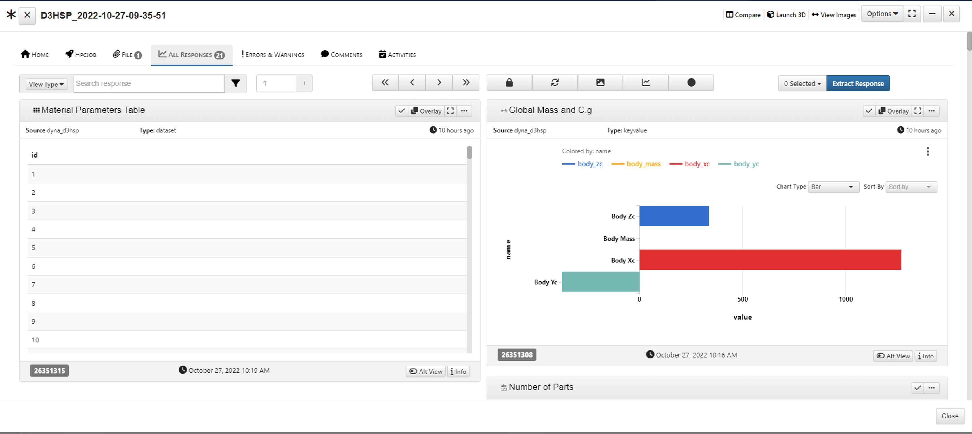
Figure 31: d3hsp Material Details Responses
Keyword Count
For this set-up, we’ve chosen d3hsp for the file name, Keyword Count for the file type and named the response.

Figure 32: d3hsp Keyword Count
This extraction gives us an individual response for Keyword Count.
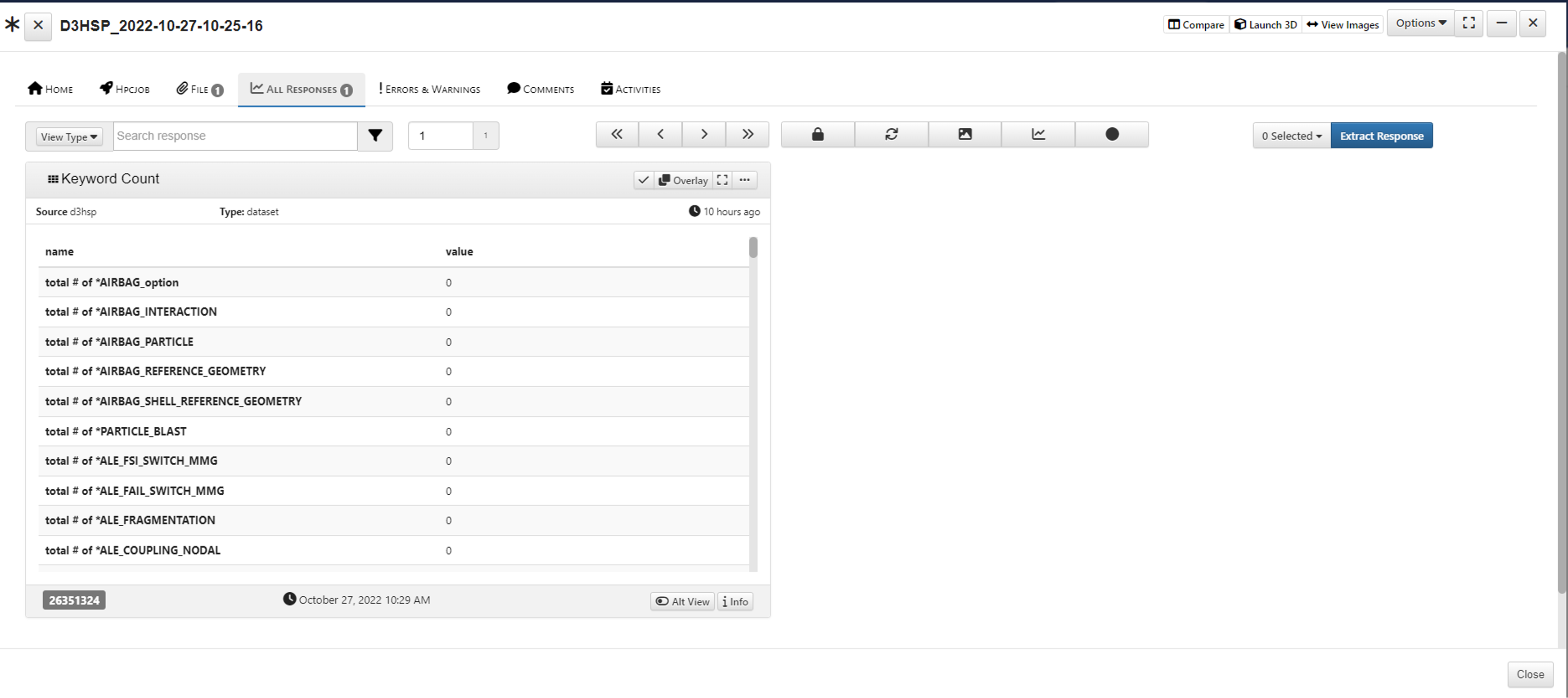
Figure 33: d3hsp Keyword Count Responses
Contacts Summary
For this set-up, we’ve chosen d3hsp for the file name, Contacts Summary for the file type and named the response.
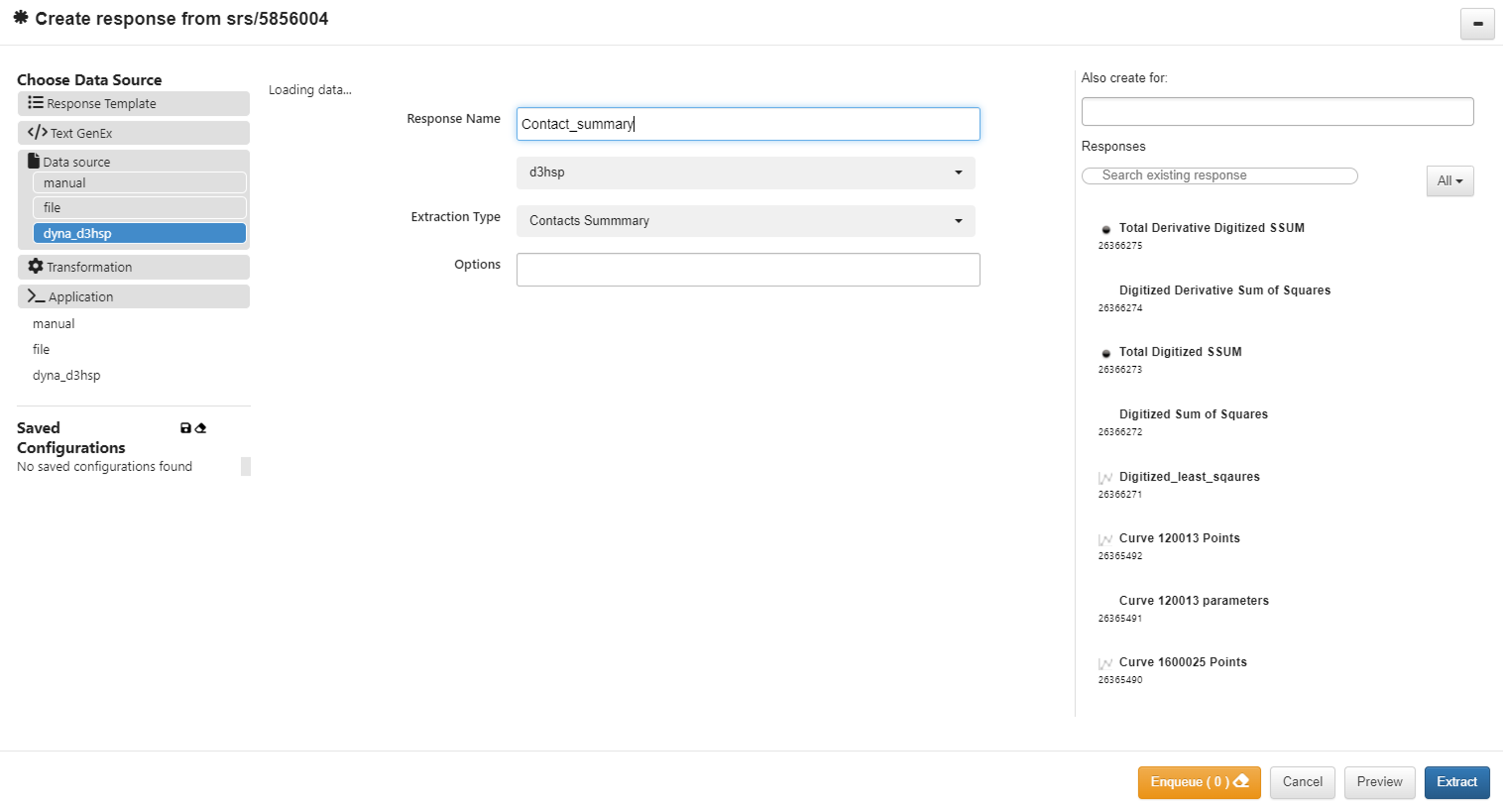
Figure 34: d3hsp Contacts Summary
This extraction gives us an individual table response for Contacts Summary.
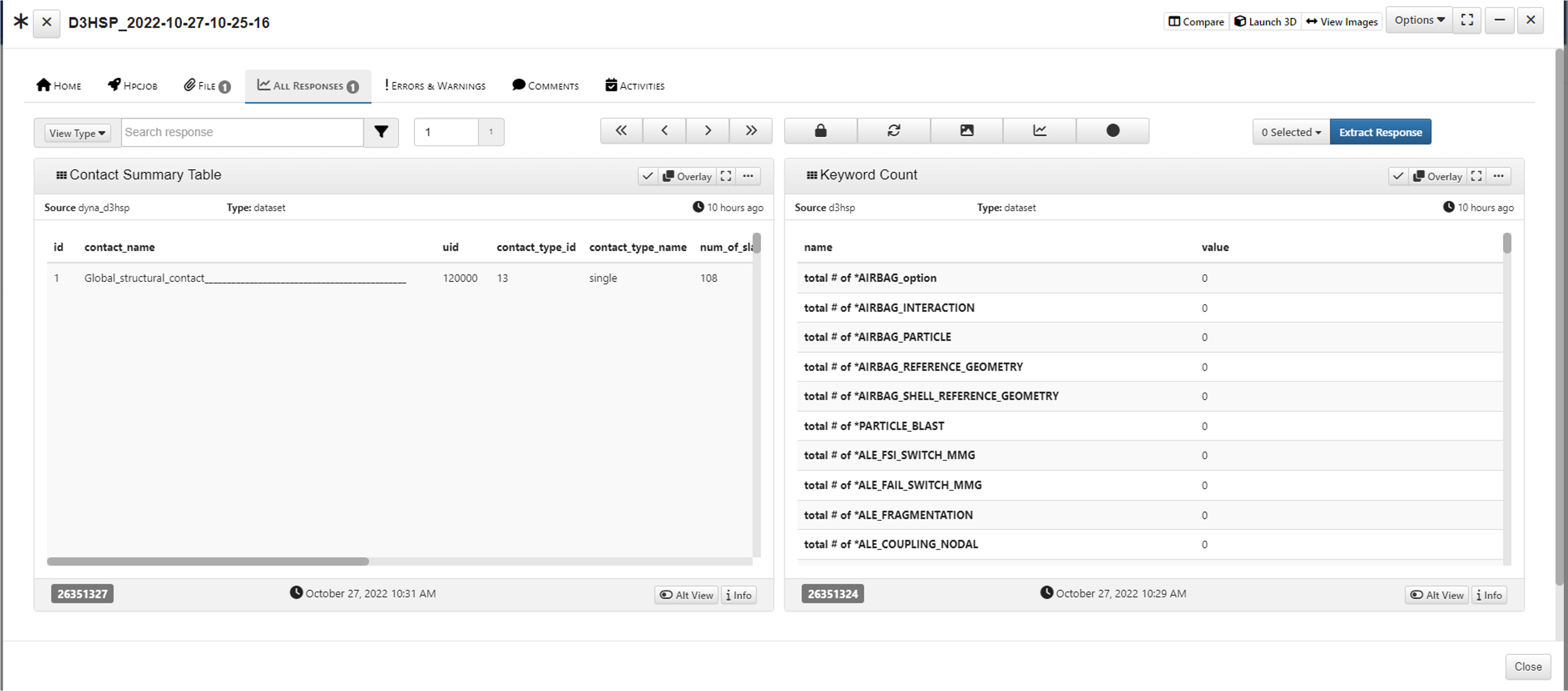
Figure 35: d3hsp Contacts Summary Responses
Contacts Parameters
For this set-up, we’ve chosen d3hsp for the file name, Contacts Parameters for the file type and named the response.
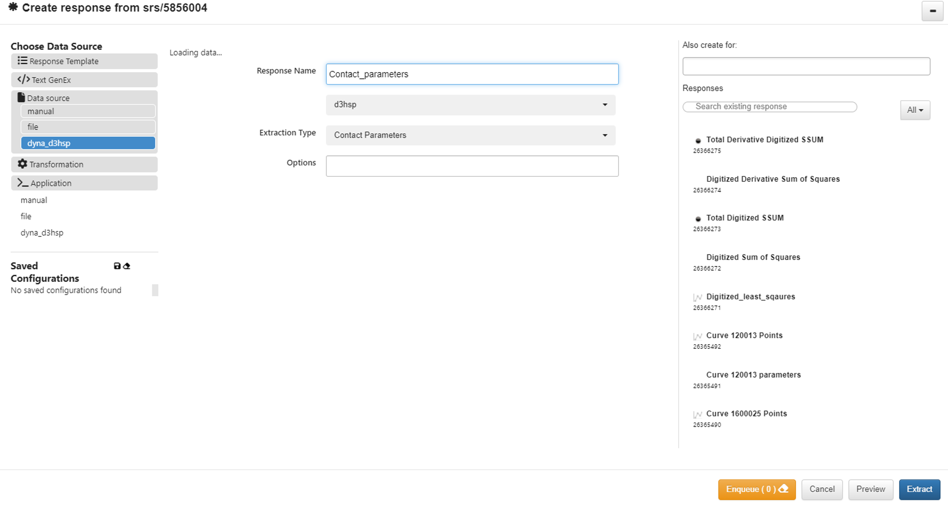
Figure 36: d3hsp Contacts Parameters
This extraction gives us an individual table response for Contacts Parameters.
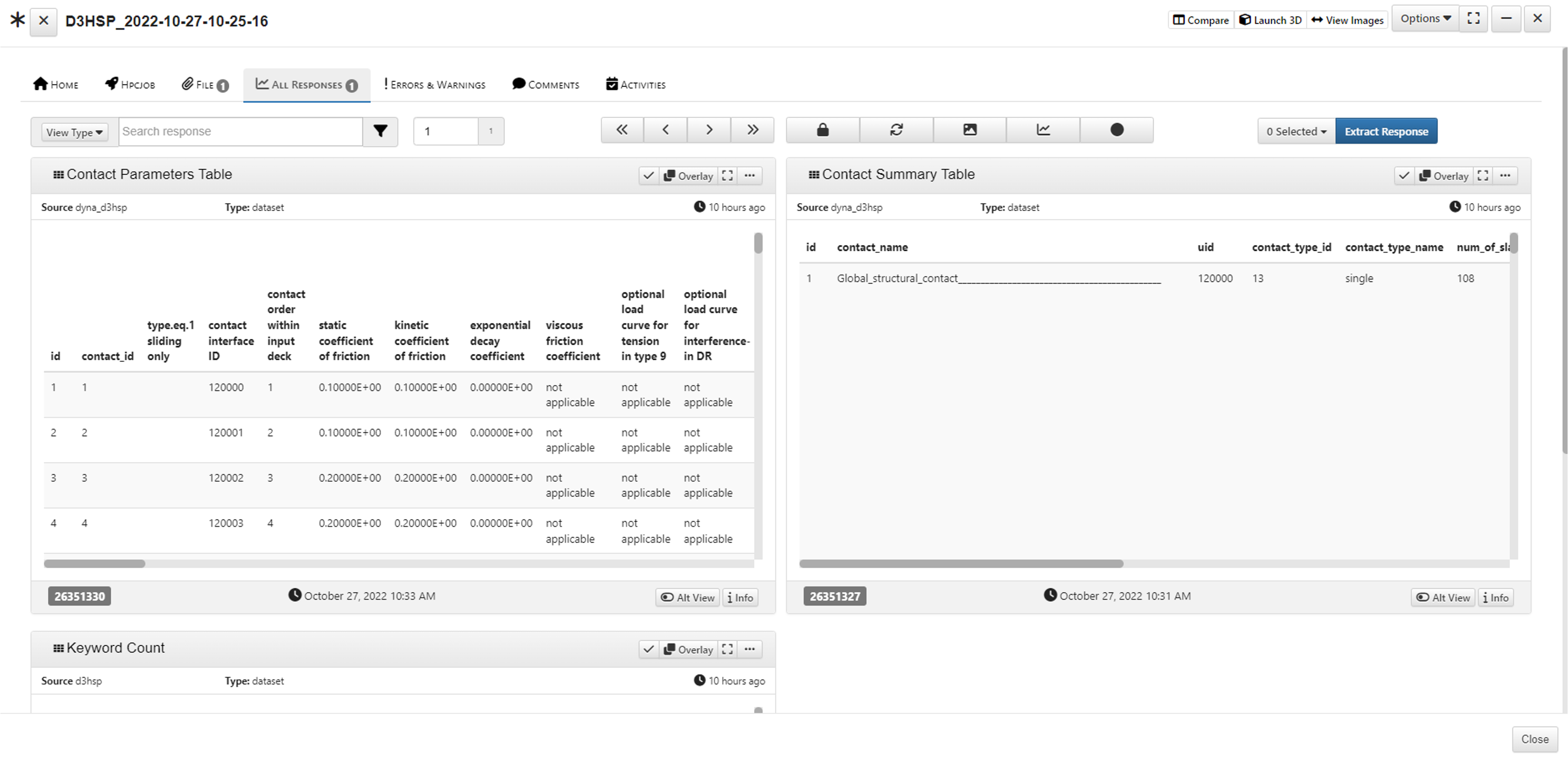
Figure 37: d3hsp Contacts Parameters Responses
Curve By ID
For this set-up, we’ve chosen d3hsp for the file name, Curve By ID for the file type and named the response.
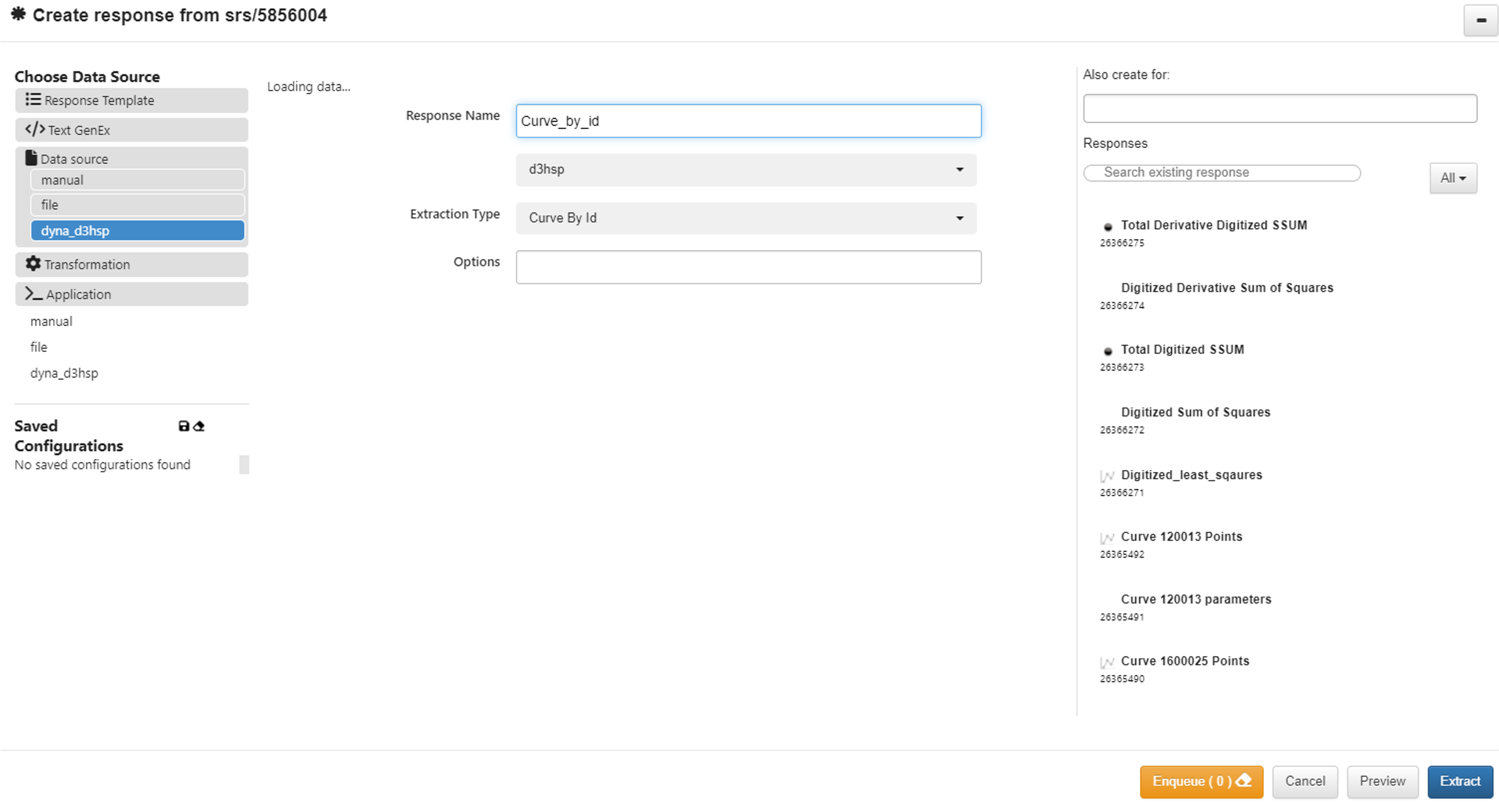
Figure 36: d3hsp Curve By ID
This extraction gives us individual curve responses by ID.
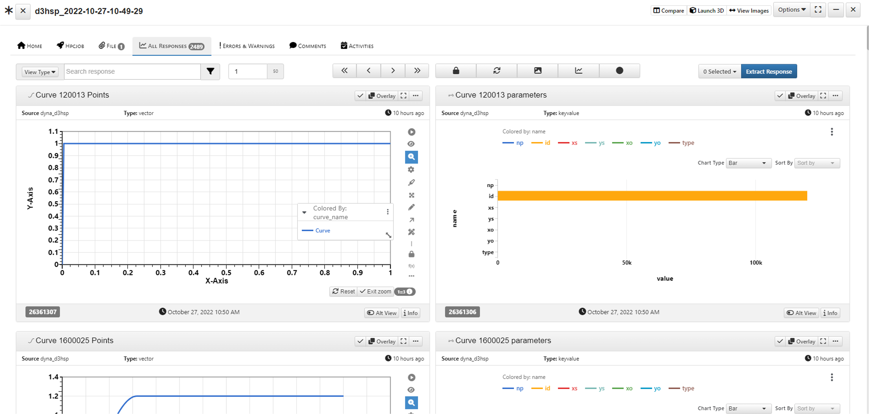
Figure 37: d3hsp Curve By ID Responses
Digitized Curves
For this set-up, we’ve chosen d3hsp for the file name, Digitized Curves for the file type and named the response.
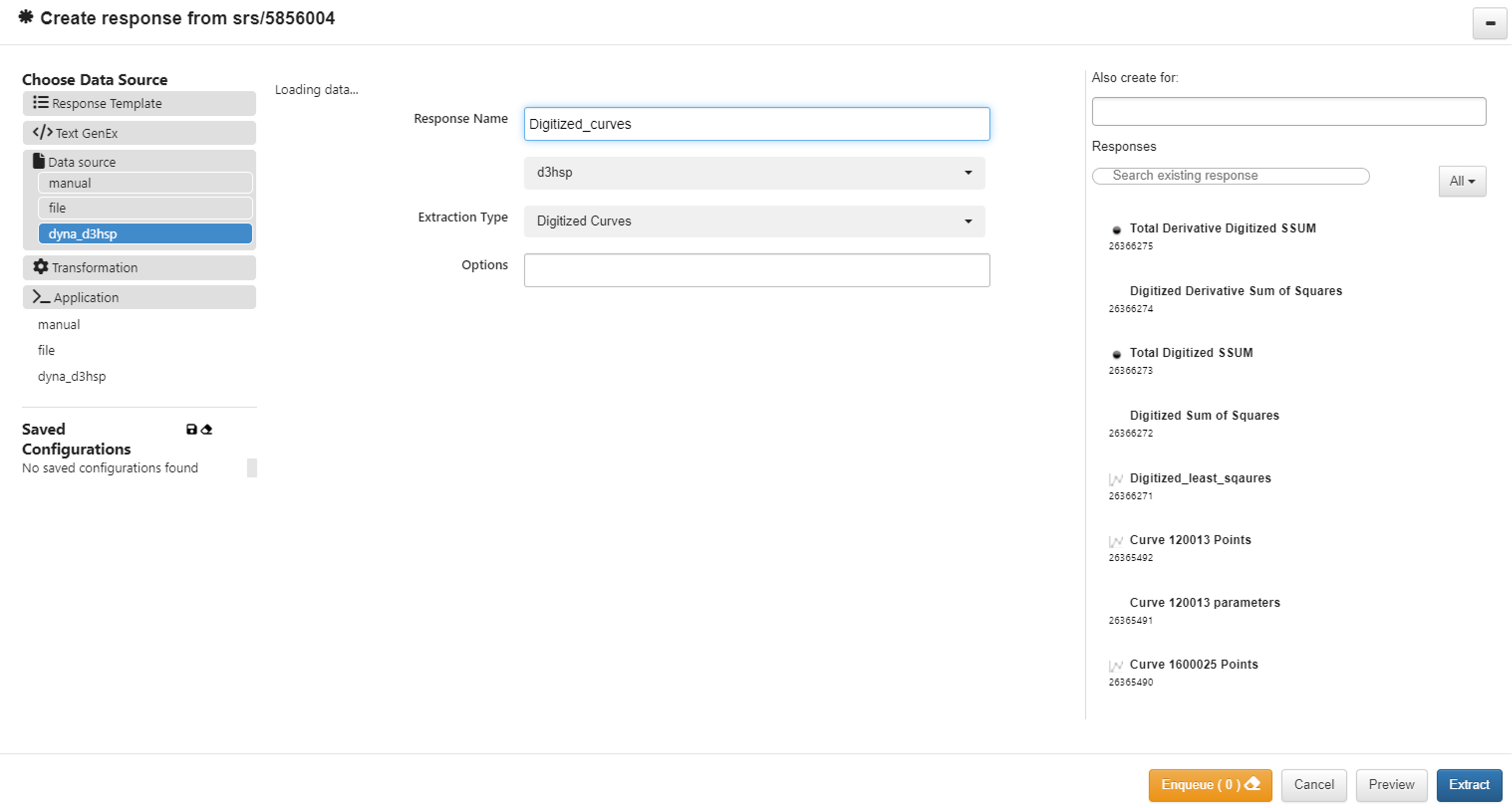
Figure 38: d3hsp Digitized Curves
This extraction gives us individual digitized curve responses.
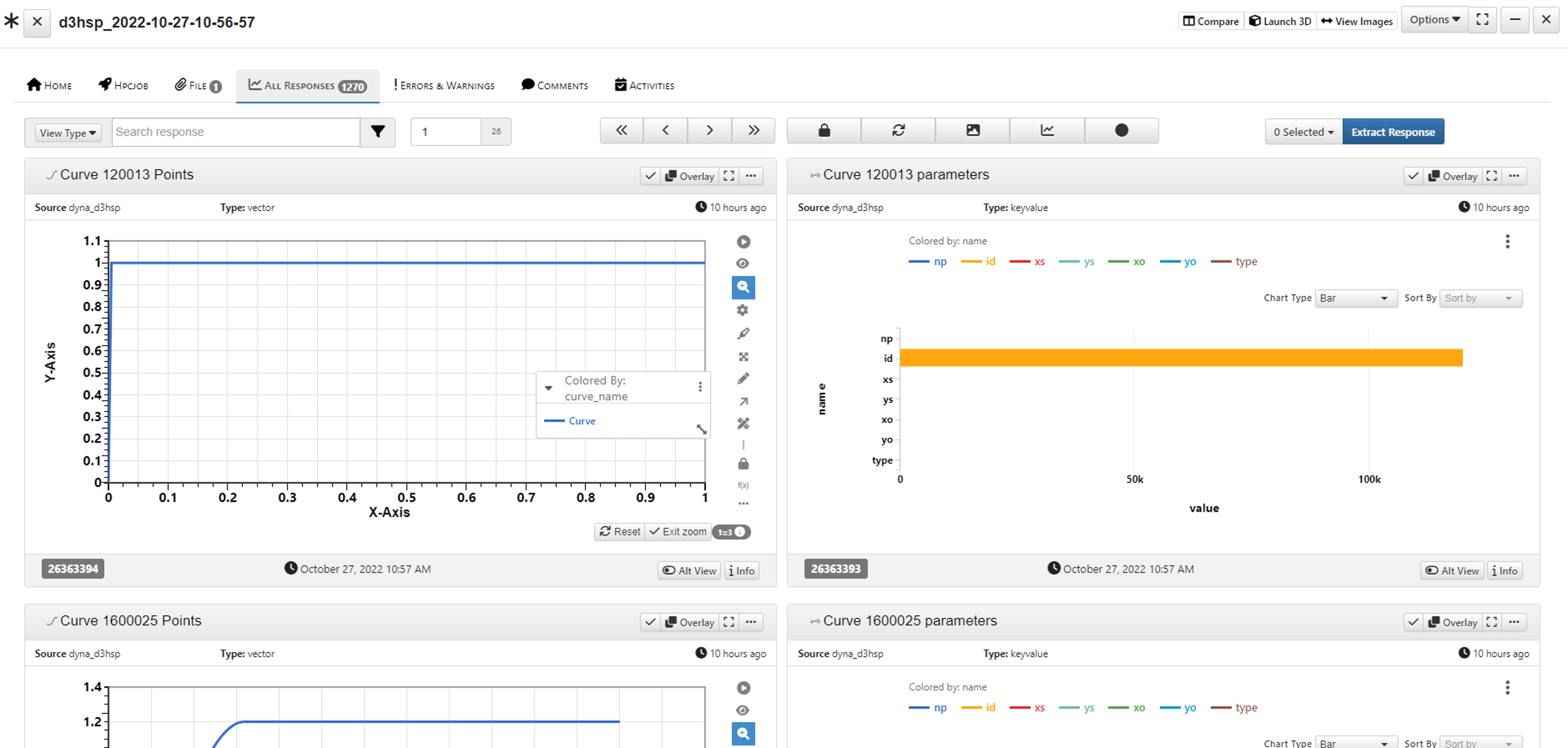
Figure 39: d3hsp Digitized Curves Responses
nastran_pch Extractor
The nastran_pch extractor uses a data source from a NASTRAN simulation for response creation.
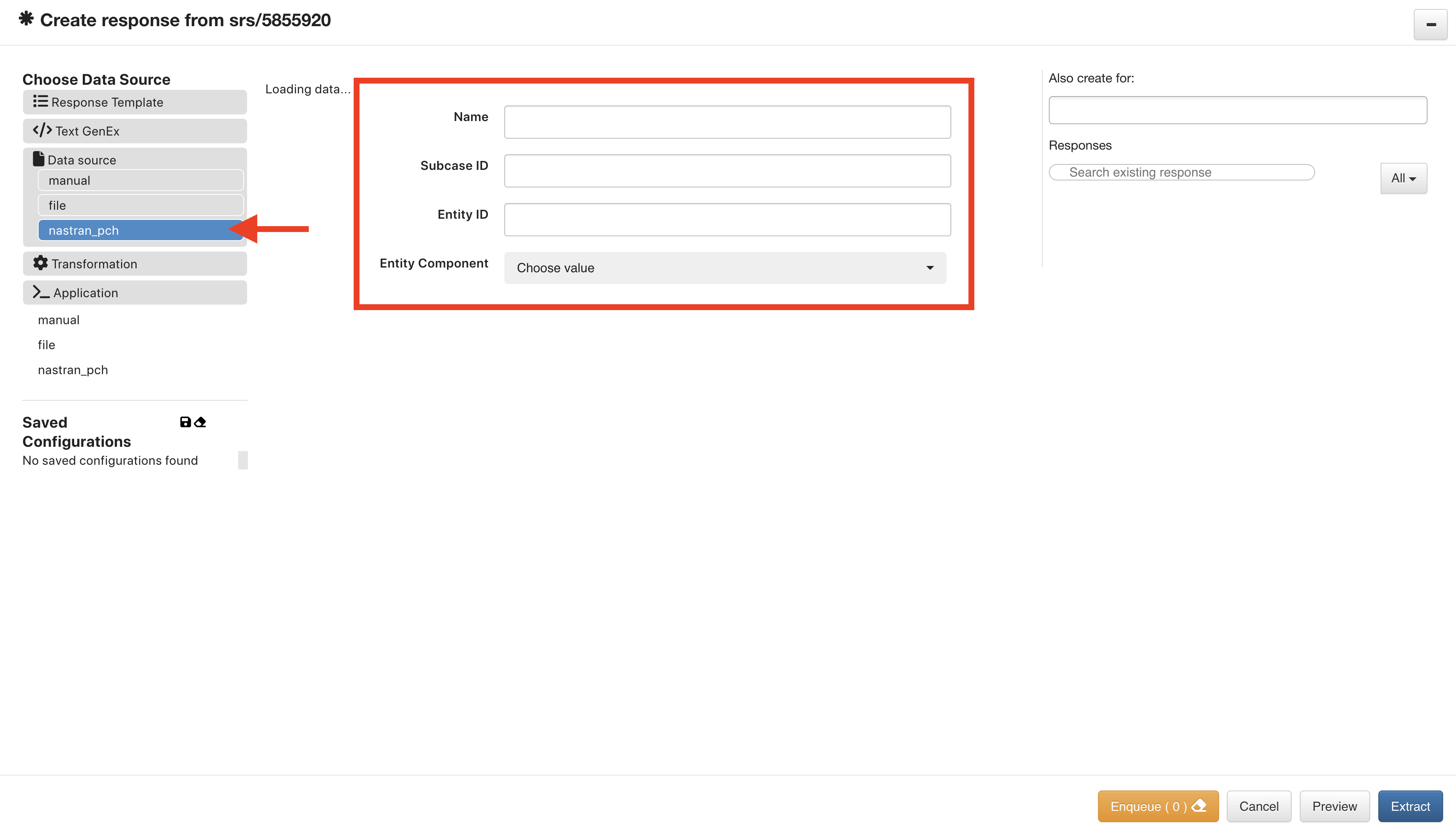
Figure 40: nastran_pch Extractor
Let’s review an example of extracting a response for a NASTRAN simulation. When setting up the extraction, we’ll want to indicate the subcase ID (1), entity ID (2) and entity component (3) as well as give the response a suitable name (4).
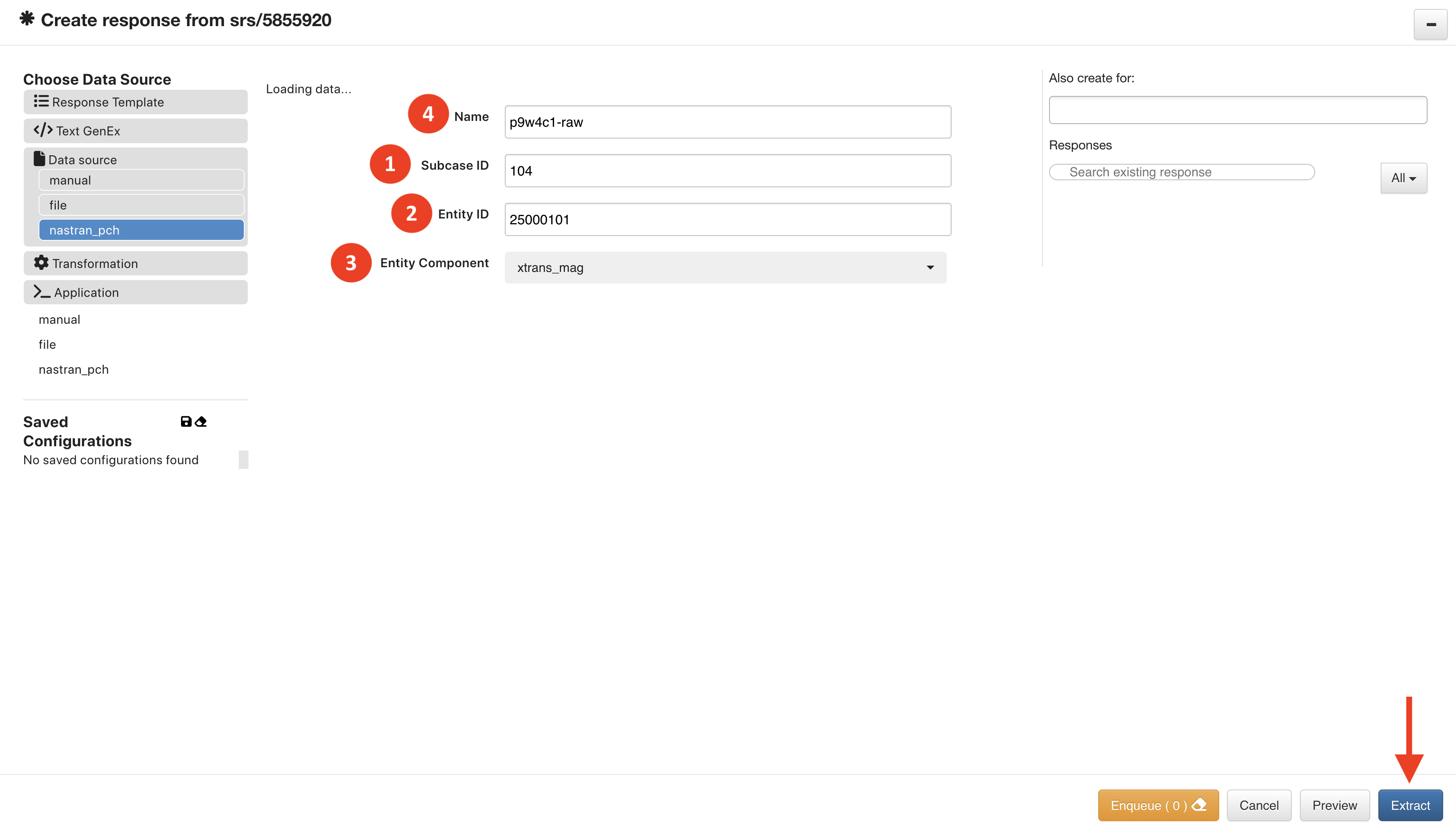
Figure 41: nastran_pch Extractor
Upon extraction, we’ll see the new response in the simulation, this one being a raw curve.
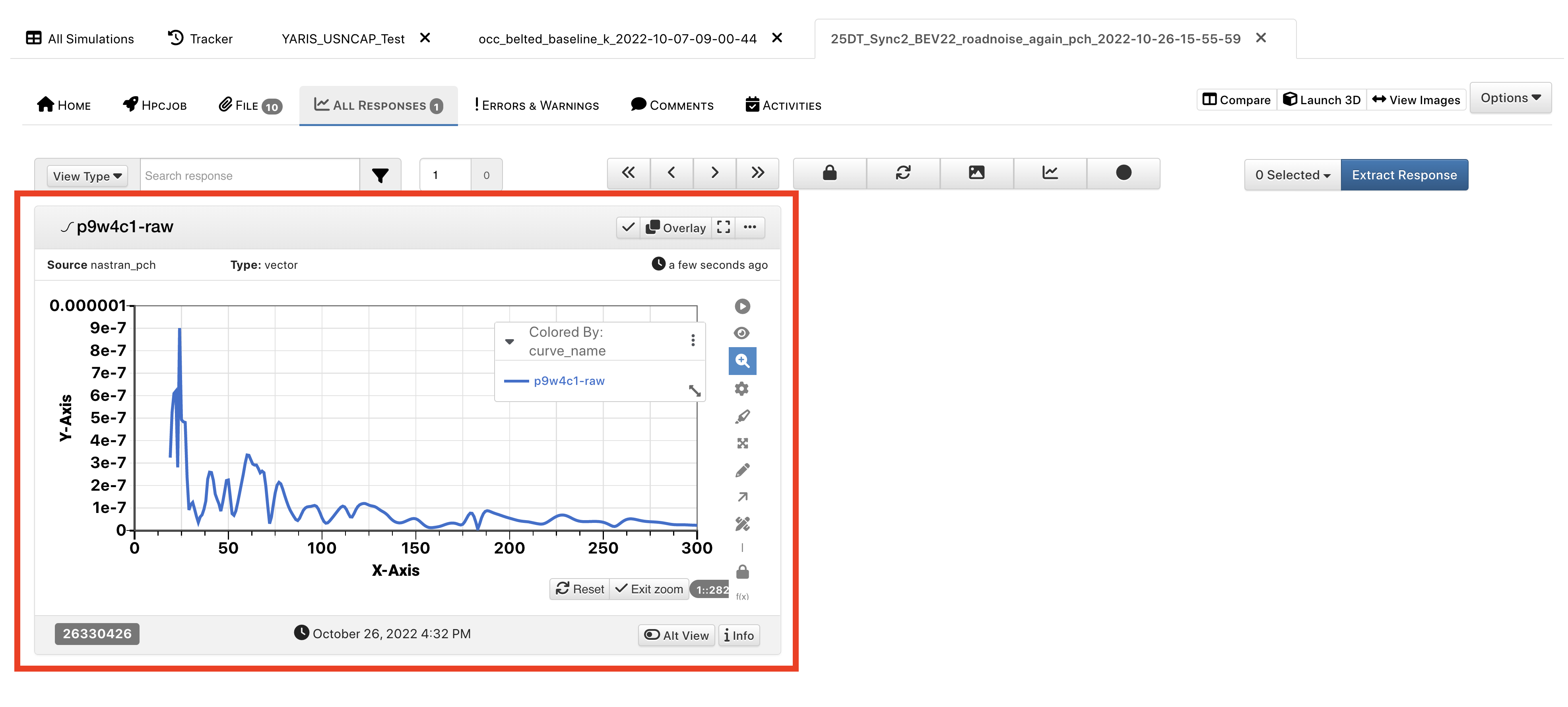
Figure 42: nastran_pch Extracted Response
We can extract more responses using the nastran_pch extractor or use dedicated template. Here is an example of responses in a NASTRAN template with the one created above indicated with an arrow. To learn more about Templates, c:ref:check out that section here. <Templates>
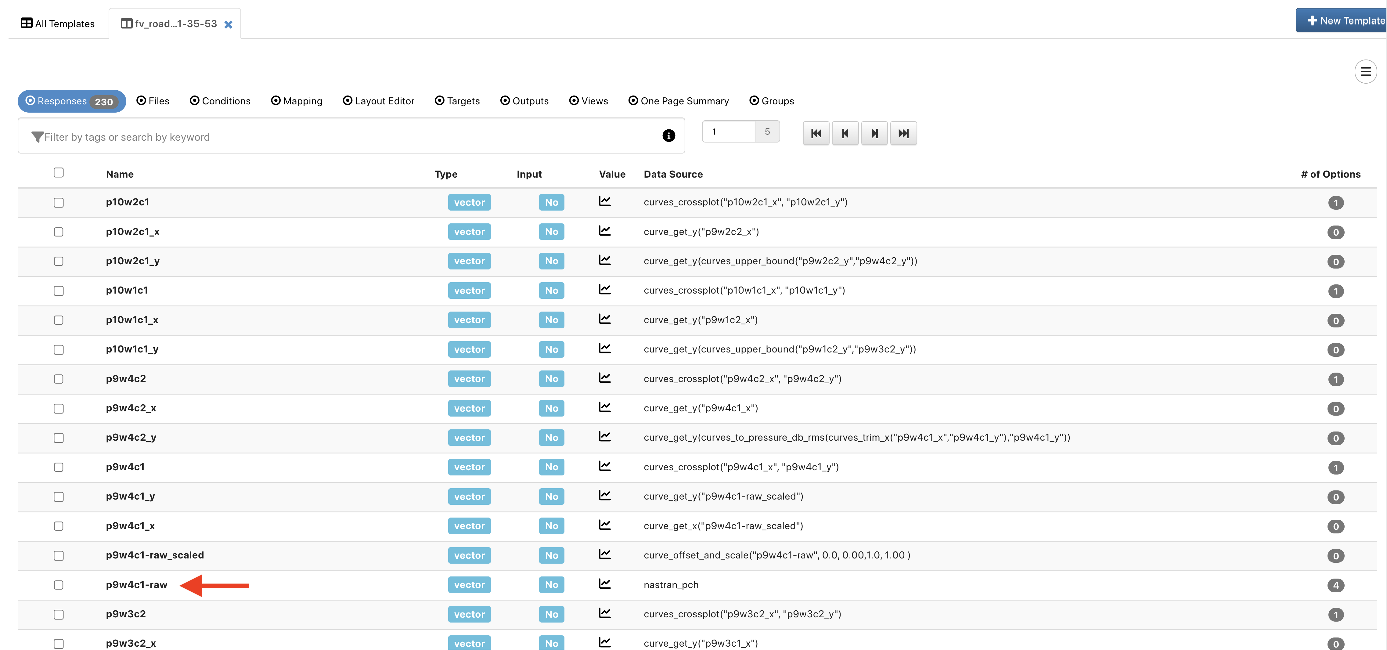
Figure 43: NASTRAN Response Template
Transformations
Applying transformations to simulation data involves employing a worker to a current simulation response. There are multiple ways to apply transformations, but the easiest way is to choose the worker from the Simple menu.
Figure 44: Simple Transformation
We can search for our desired worker or use the drop-down menu to sift through categories.
Choosing A Worker
Click on your desired worker to see it’s inputs. Here, we’ve chosen curve_reversepoints.
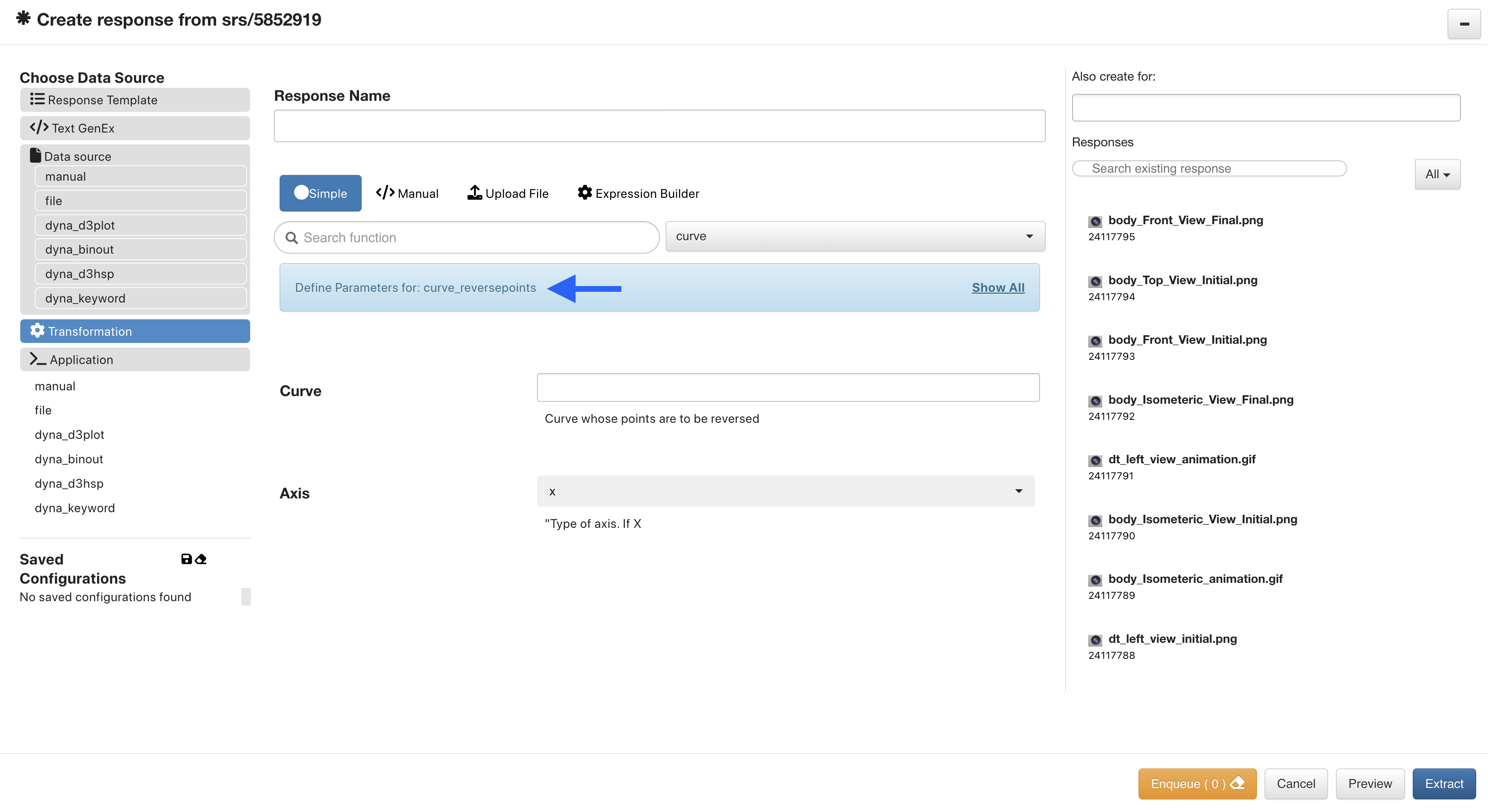
Figure 45: Choose Worker
Then, we’ll drag-and-drop the curve response to be transformed from the right side menu into the curve input and choose which axis to reverse.
Curve Reverse Points Set-Up
6.9. Simulation Mid-Run Extraction
NEW as of June 7, 2022: You can now extract stale/delete-and-extract/and extract transformations only. This avoids the need to manually remove old responses for a solving simulation.
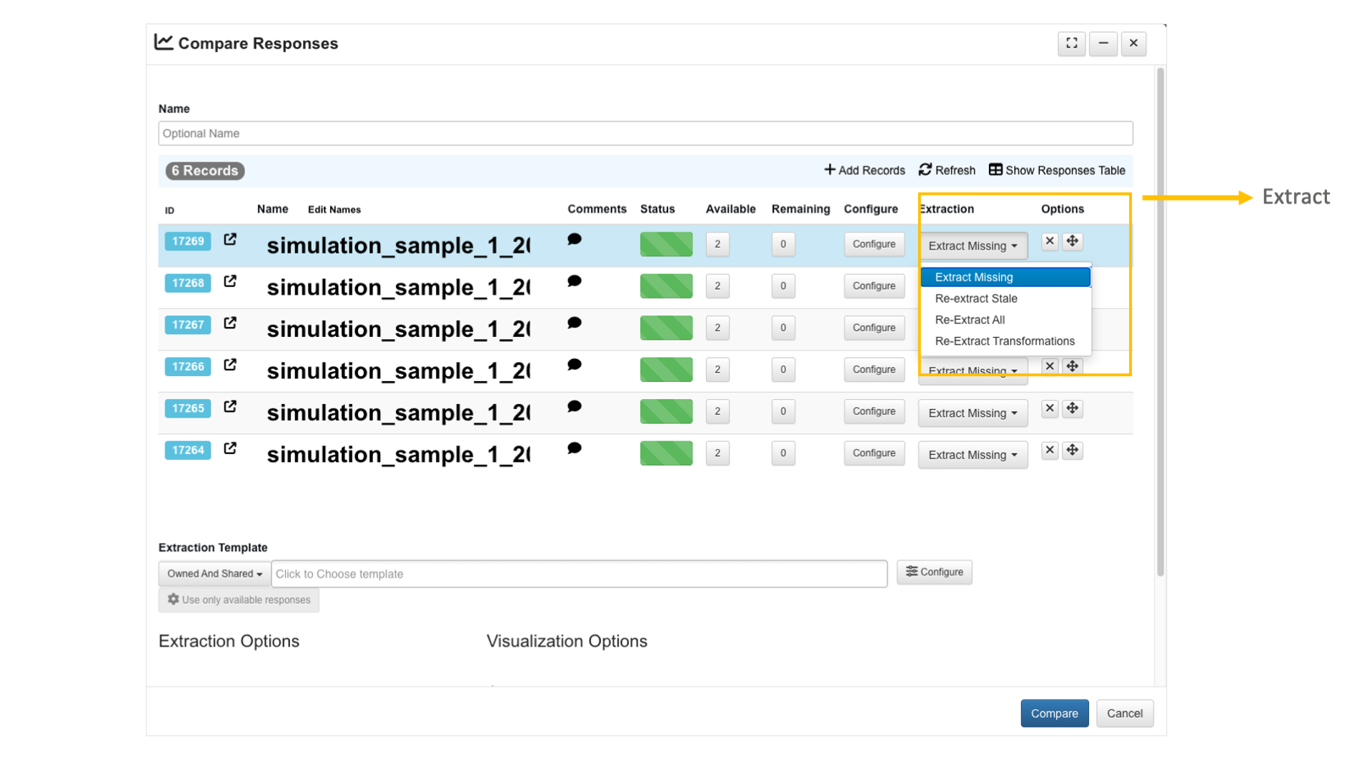
Figure 1: Mid-Run Extraction
Here is an example:
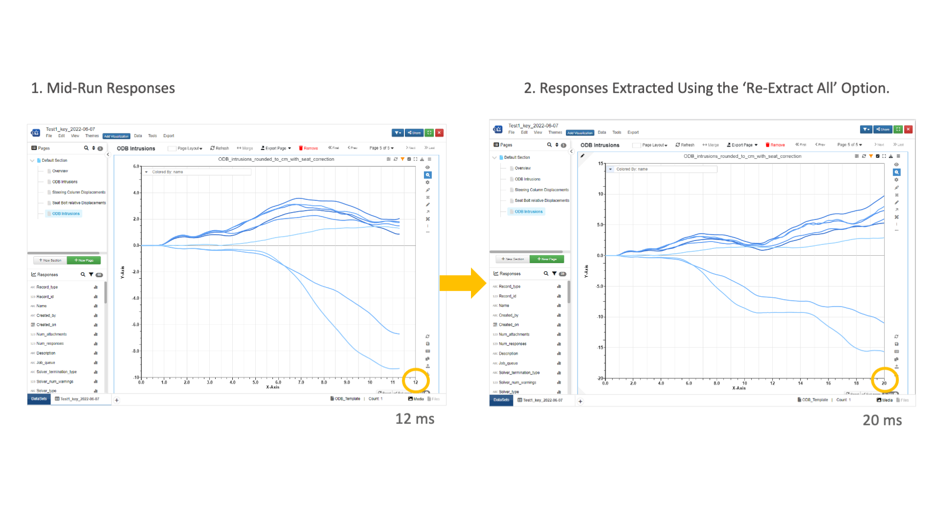
Figure 2: Mid-Run Extraction Example
You can also use the refresh button if there are more responses to be extracted.
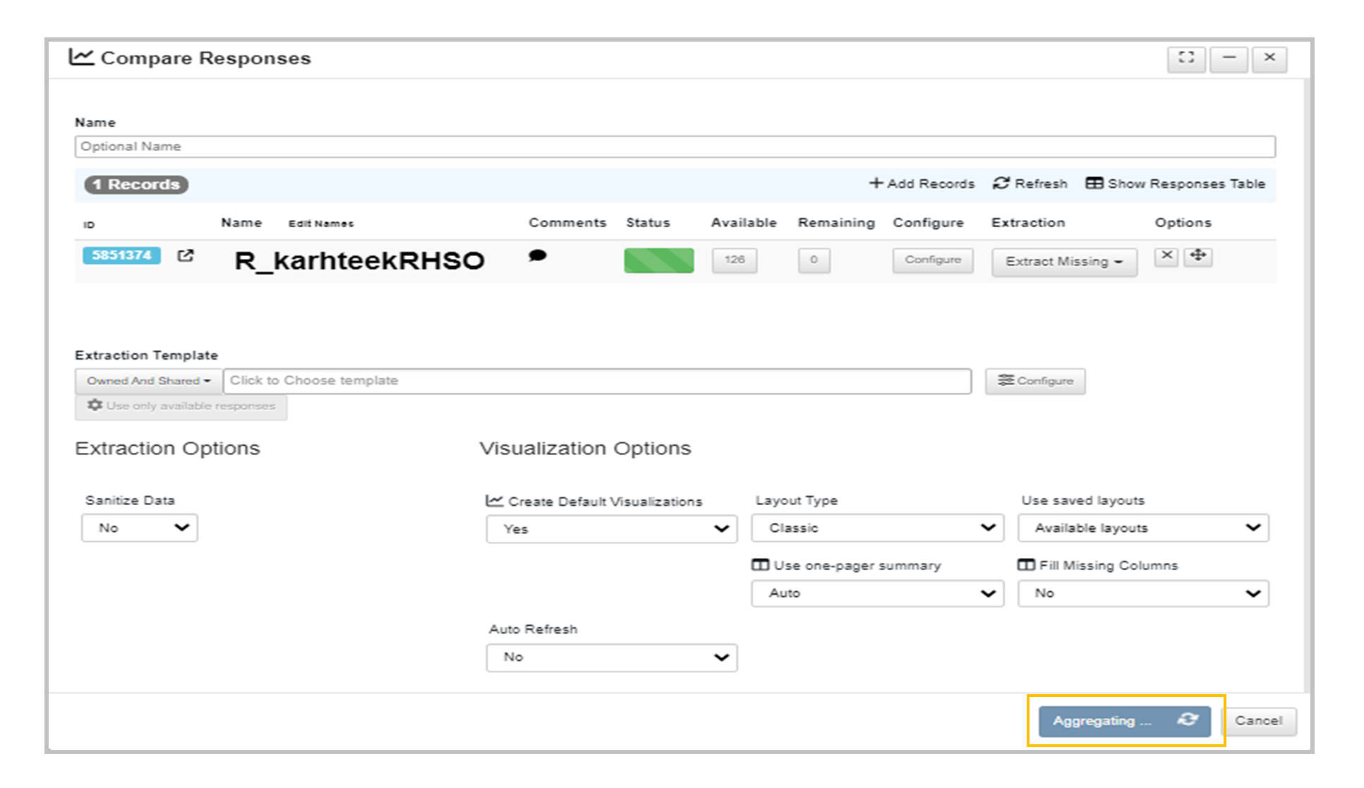
Figure 3: Refresh button
These options refresh data applied for partially completed simulation.
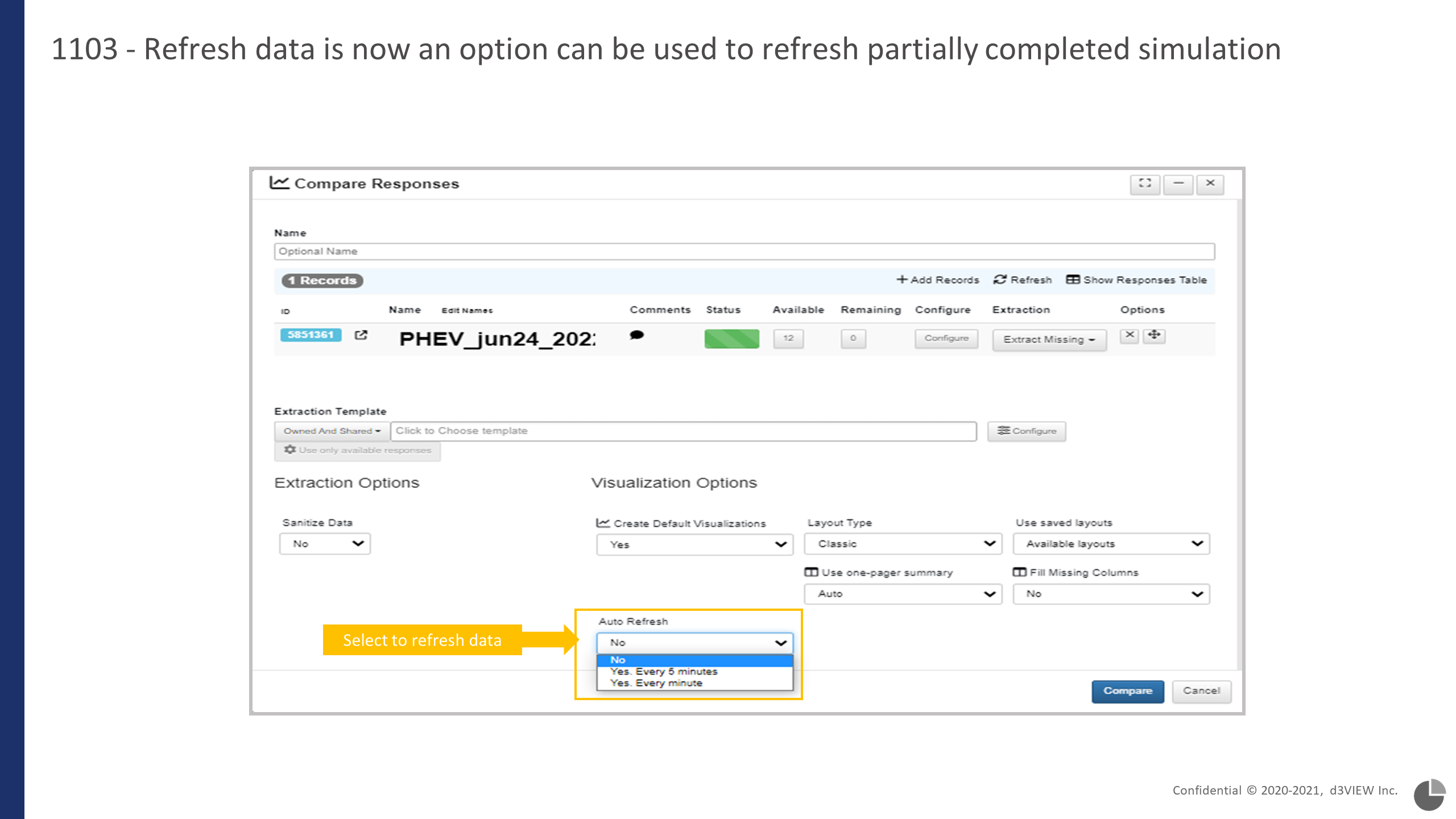
Figure 4: Refresh data
6.10. Apply Filter to a Response
How to Apply a Filter to Responses?
Right-click on the response curve
Locate the response curve in the interface. Right-click on it to open the context menu.
Select “Operate On” from the context menu
In the menu that appears, choose Operate On to access available operations.
Search for curve_filter
In the operation list search bar, type curve_filter and select it from the results.
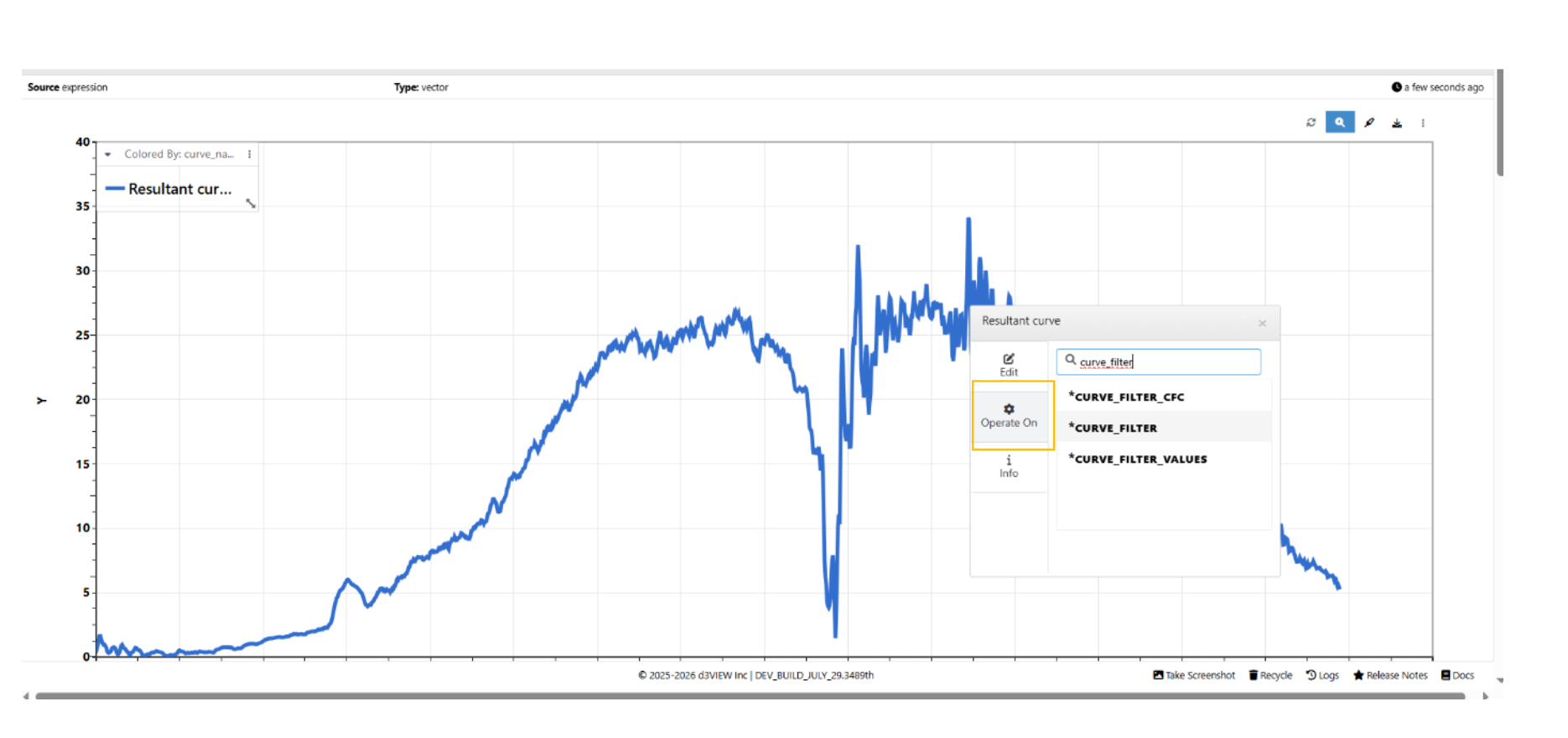
Operate On
- Choose transformation “curve_filter”.
Curve_filter
Configure the Options
Choose Filter Class: Set the filter frequency to “60” from the available options.
Adjust Additional Settings: Modify any other parameters or options according to your requirements.
Click on Apply
Curve_filter applied
- View the Filtered Response Curve

Filtered Curve
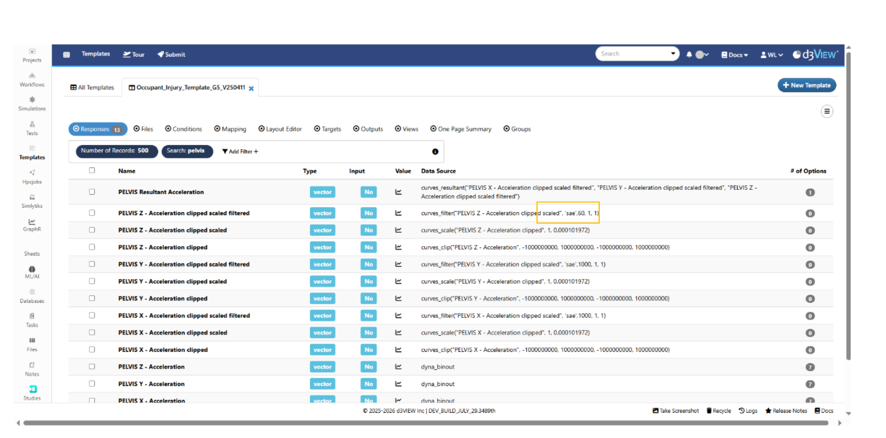
Update Filter Settings in Template
Open Template
Click on the “Template” Icon
Locate and click the Template icon to open the Template Application.
Search for the Template
Use the search bar or filter options to find the template you want to update.
Click on the Template Name
From the search results or the list of templates, click the template name to open it for editing.
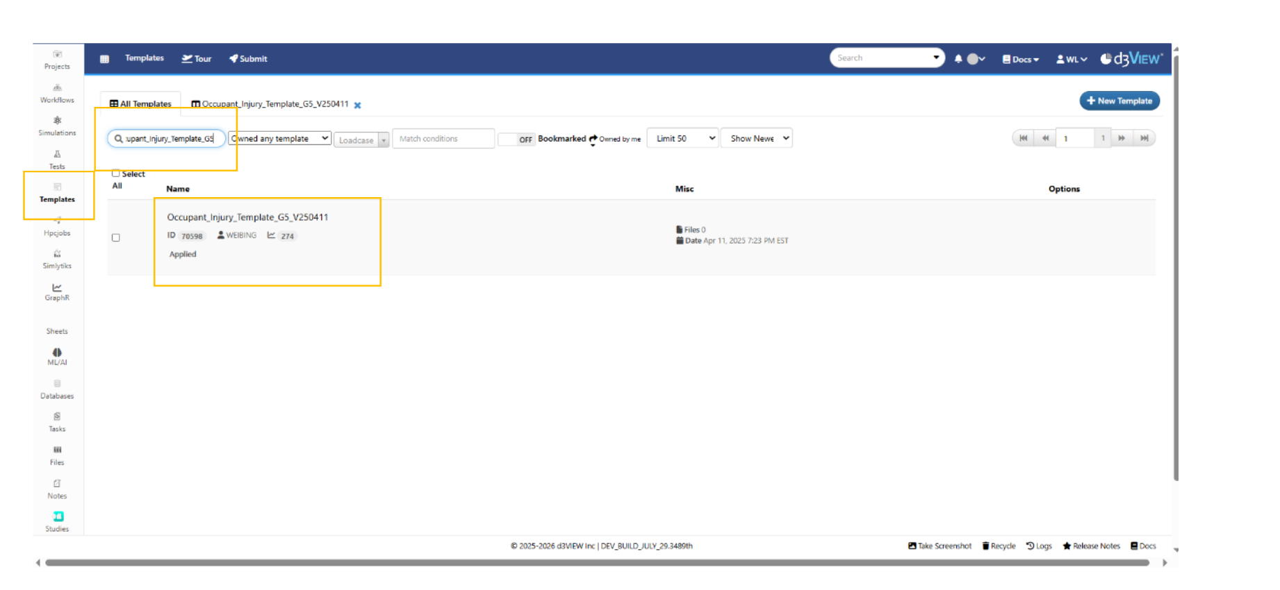
Template Search
- Click on “Filter” and choose “Number of Records”
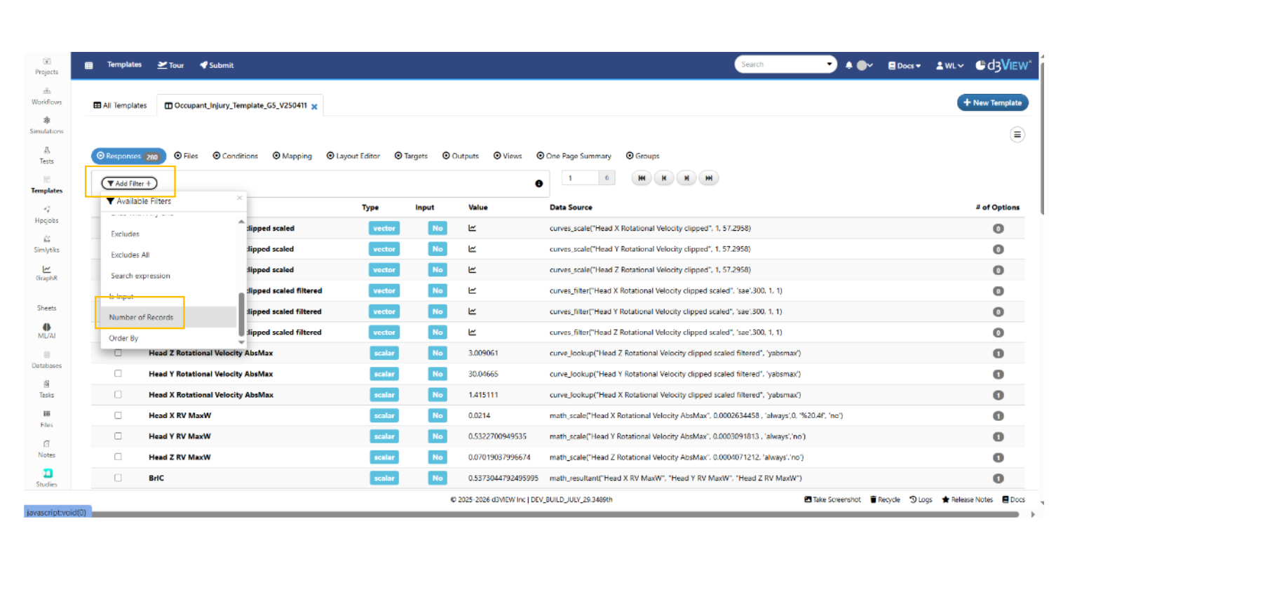
Number of records
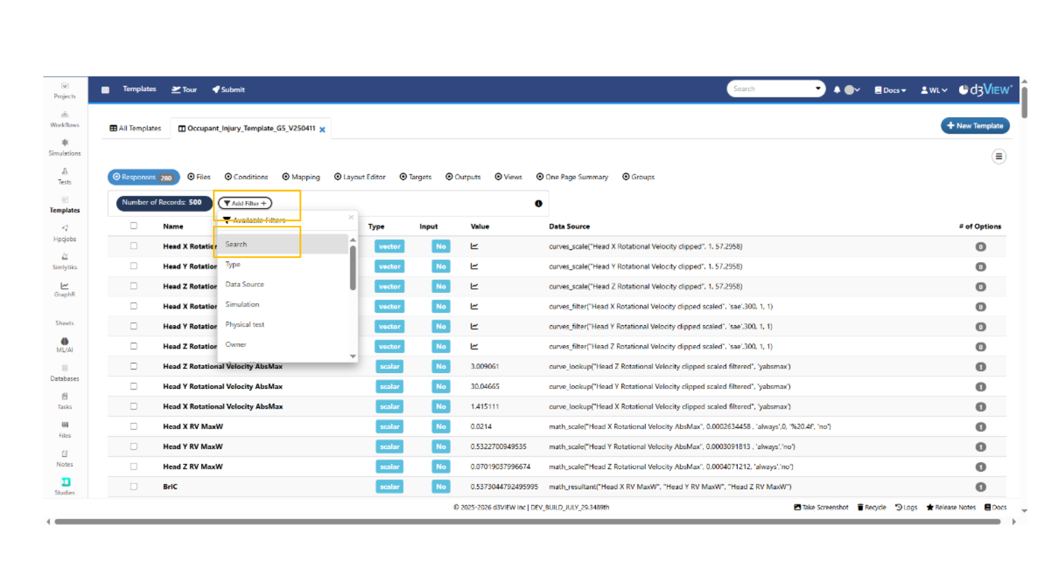
- Change the number of records to “500”

Number of records 500
- Then, Add “search” filter
- Click on “Add Filter”
- Choose “Search
- Type in keyword
- Responses having the keyword will show up.
Serach Filter
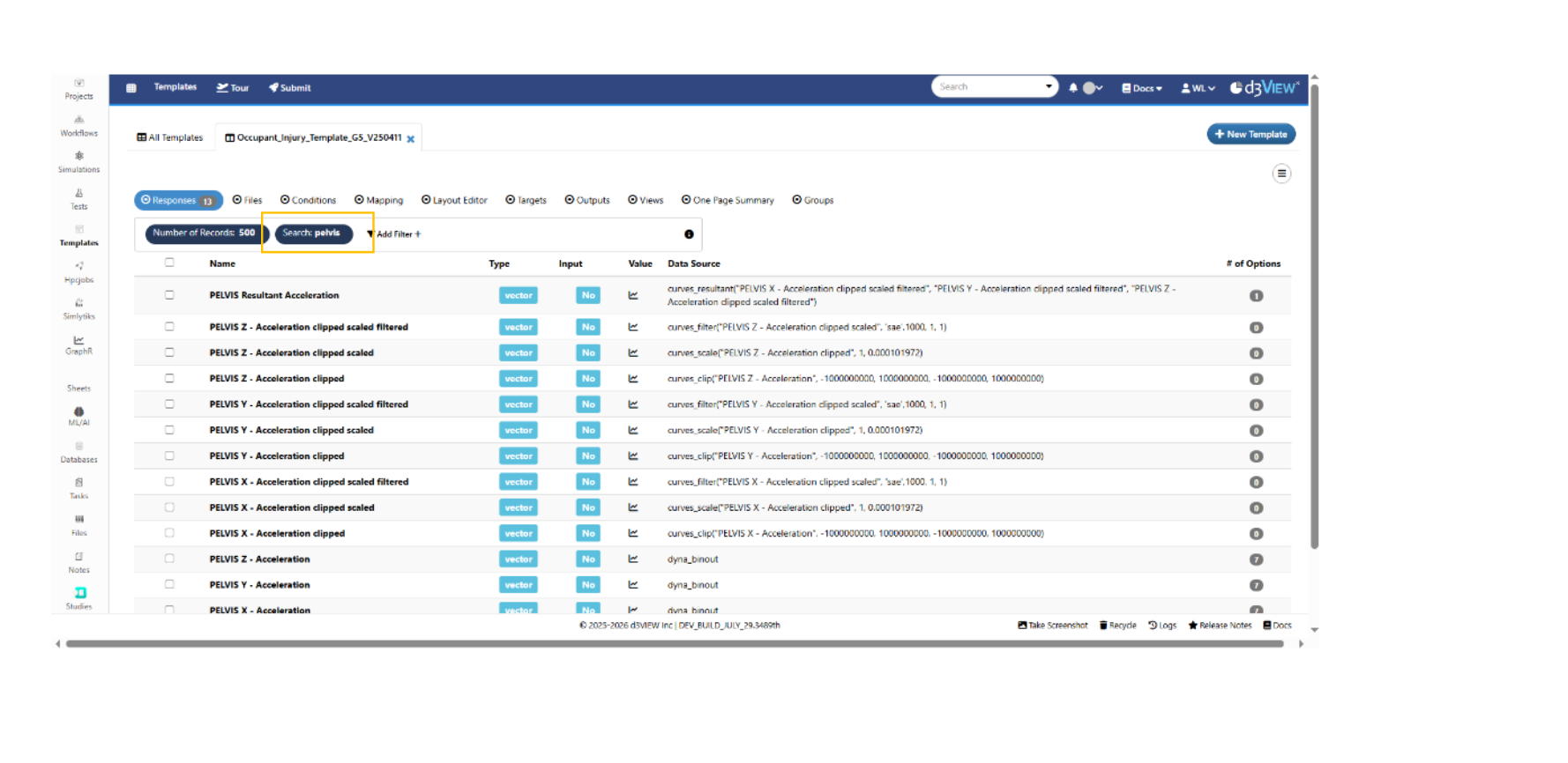
Serach Filter
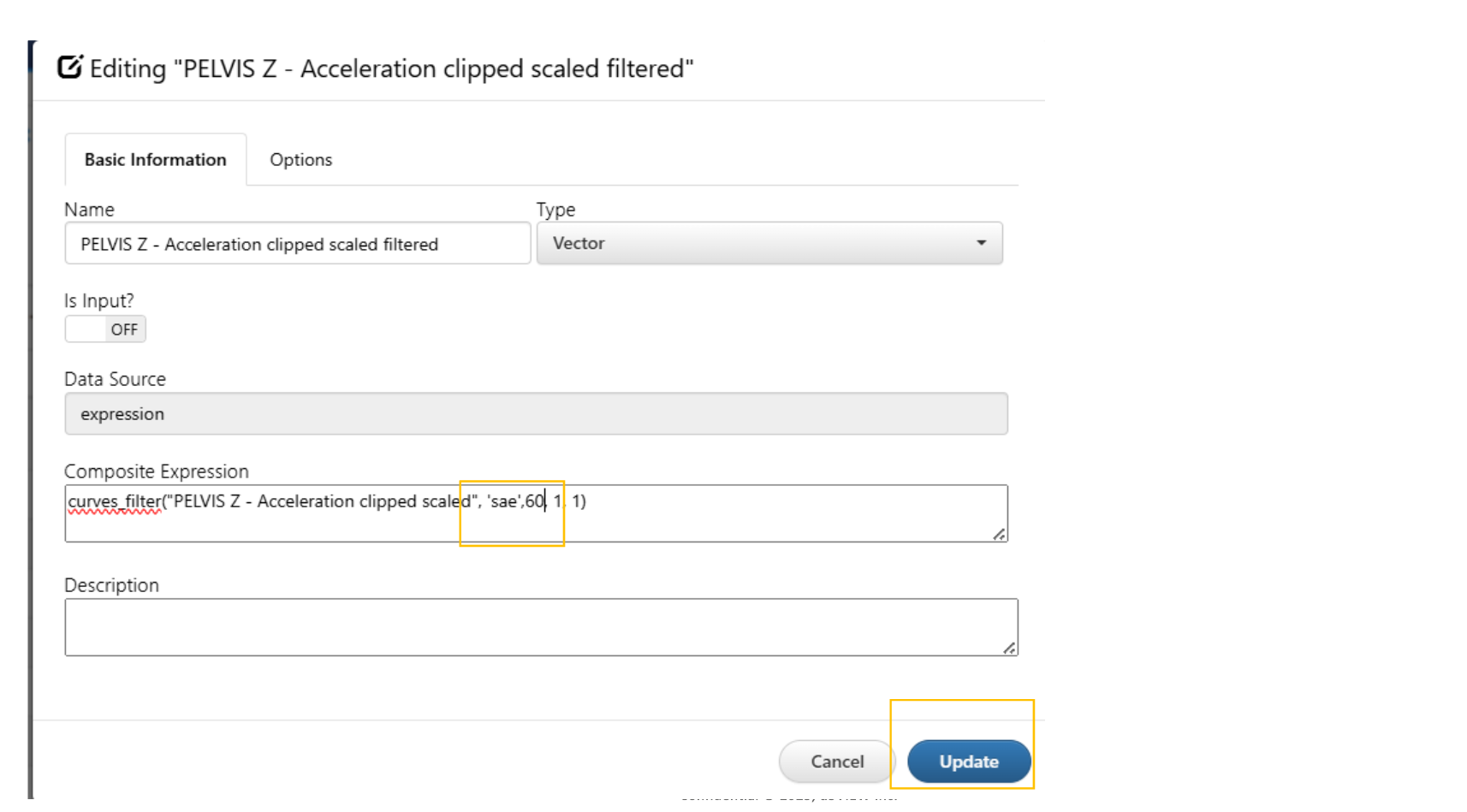
- Update Expression in Template
- Locate the Filter Expression
- Update the Filter Class : Change the filter class value to 60.
- Save the Changes
Update template
Update and Refresh Template.
Update the Template
After making changes to the filter expression or settings, click Update/Save to apply the changes.
Refresh the Page
Reopen the Template: Navigate back and open the template again to verify the changes.
Verify Updated Response Expression
Updated template
Re-apply Template
- Compare Responses in Simulation.
- Open the Simulation Application
- Locate the Simulation
- Right-click on the Simulation : Right-click on the simulation item to open the context menu.
- Choose “Compare Responses” : From the context menu, select Compare Responses to initiate a comparison of the simulation outputs.

Compare Responses
- Choose the template
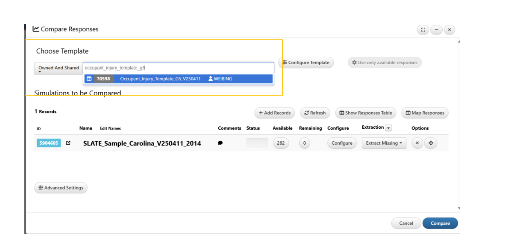
Choose Template
- Click on “Extraction” dropdown list
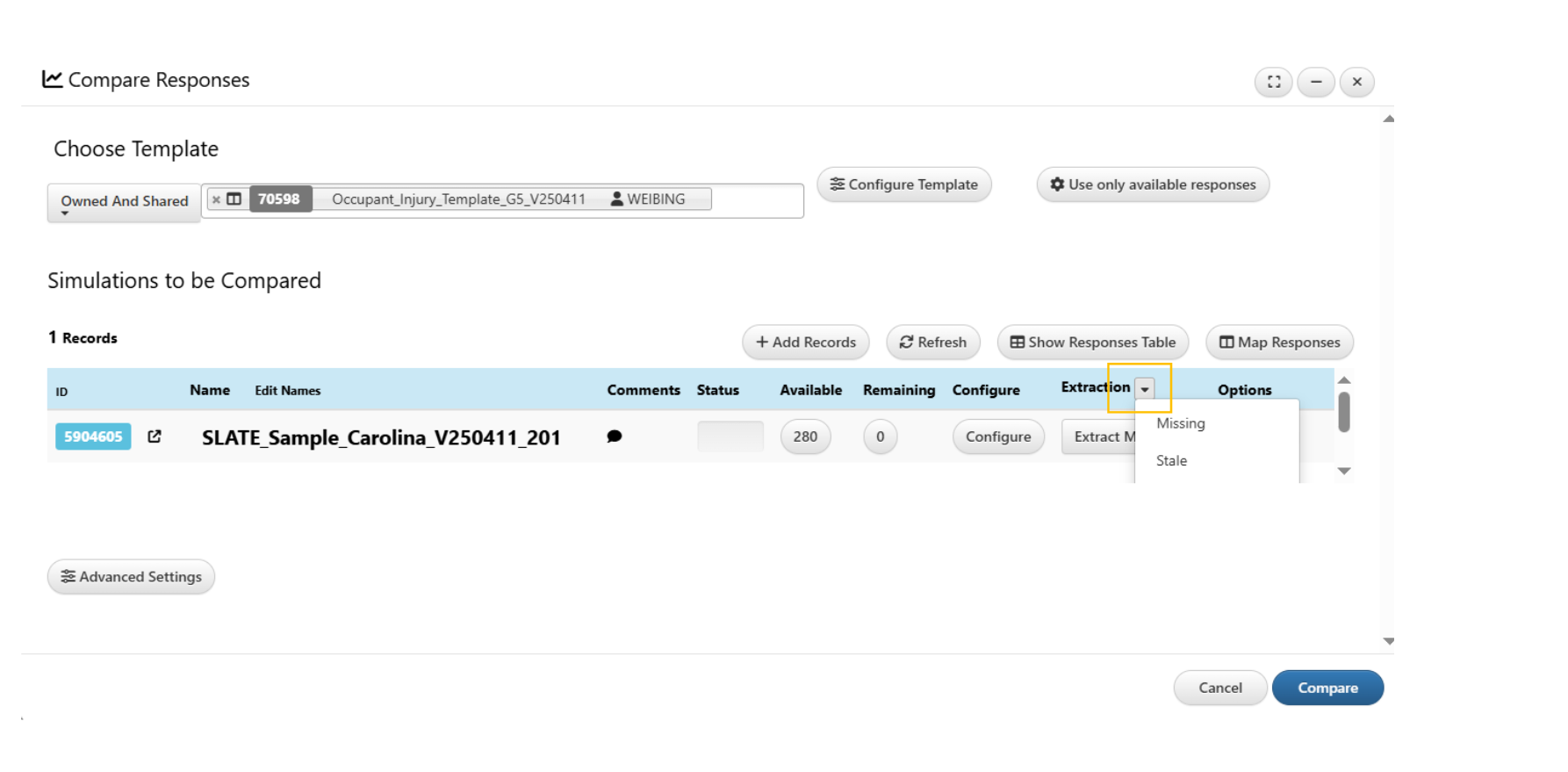
Extraction
- Scroll Down and Select “Transformation”
Extraction
- Click “Compare” to view responses in Simlytiks.
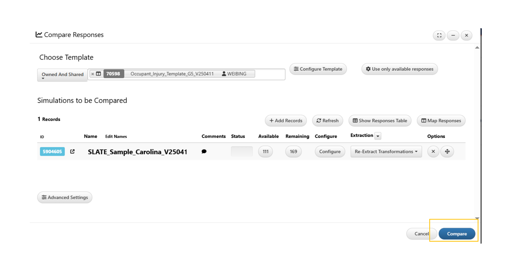
Compare
6.11. Simulation Tracker
If we are writing, editing and polishing simulations, we can create a database for tracking the run log. Let’s review.
Run Log Viewer Options
There are four different ways we can view our run log in the viewer. The following image illustrates these with examples:
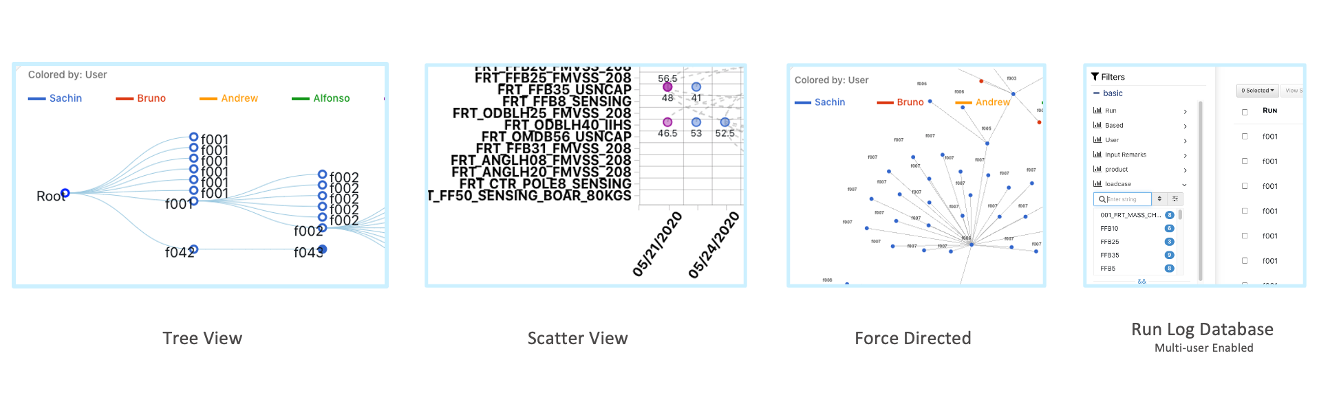
Figure 1: Run Log Viewer Options
Ways to Track Runs
There are 3 ways to track runs:
Options A – Self-managed Tracker in Excel (current practice but denormalized) Option B – Managed Manually in d3VIEW using Databases Option C - Insert from a simulation or using a Worker
Let’s go over each.
Option A
For this option, we’ll continue to maintain the Excel but in de-normalized data as shown in the example image below. We’ll then drop the file in the Simlytiks data handler to visualizer.
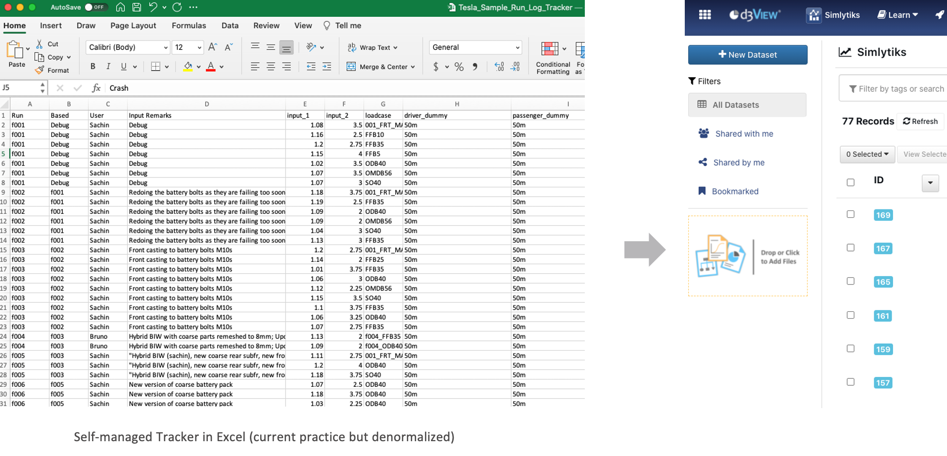
Figure 1: Option A: Self-managed Tracker in Excel
Option B
For this option, we’ll create a database in d3VIEW and manually add records.
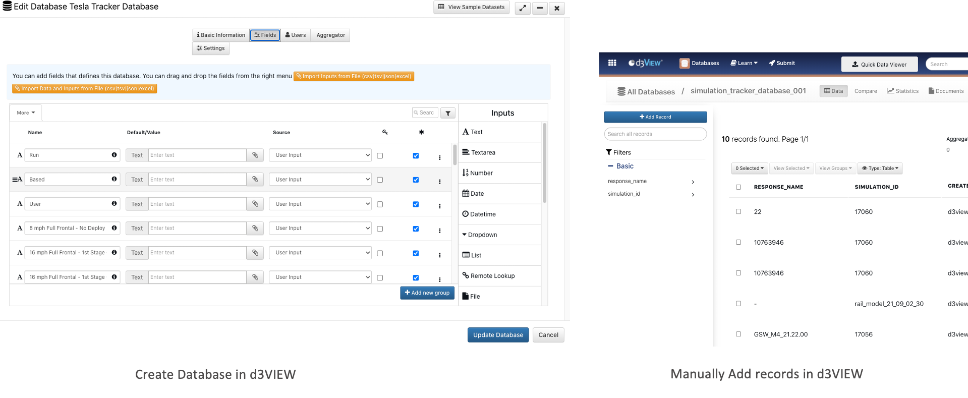
Figure 2: Option B: Managed Manually in d3VIEW using Databases
Let’s review the steps.
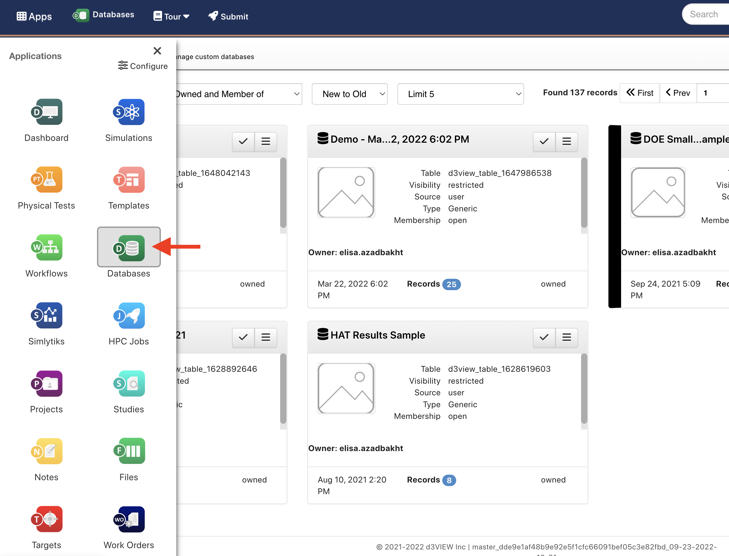
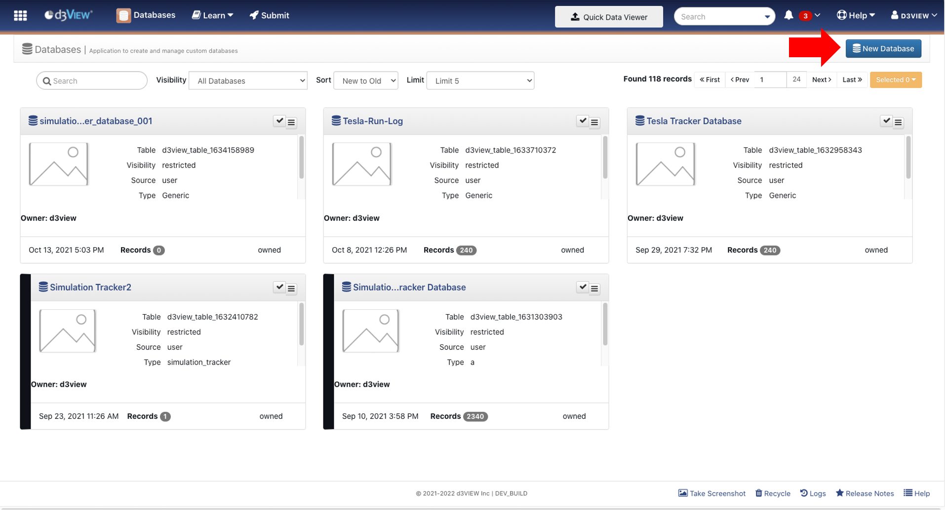
Step 1. Navigate to the Databases App
Step 2. Click on New Database
Step 3a. Input a name and some meta-data information
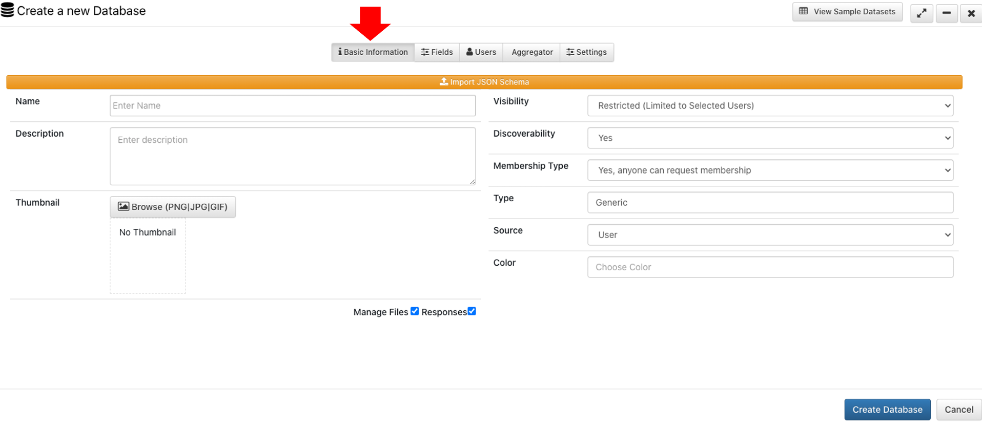
Step 3b. Define Fields by Dragging the inputs from the right menu
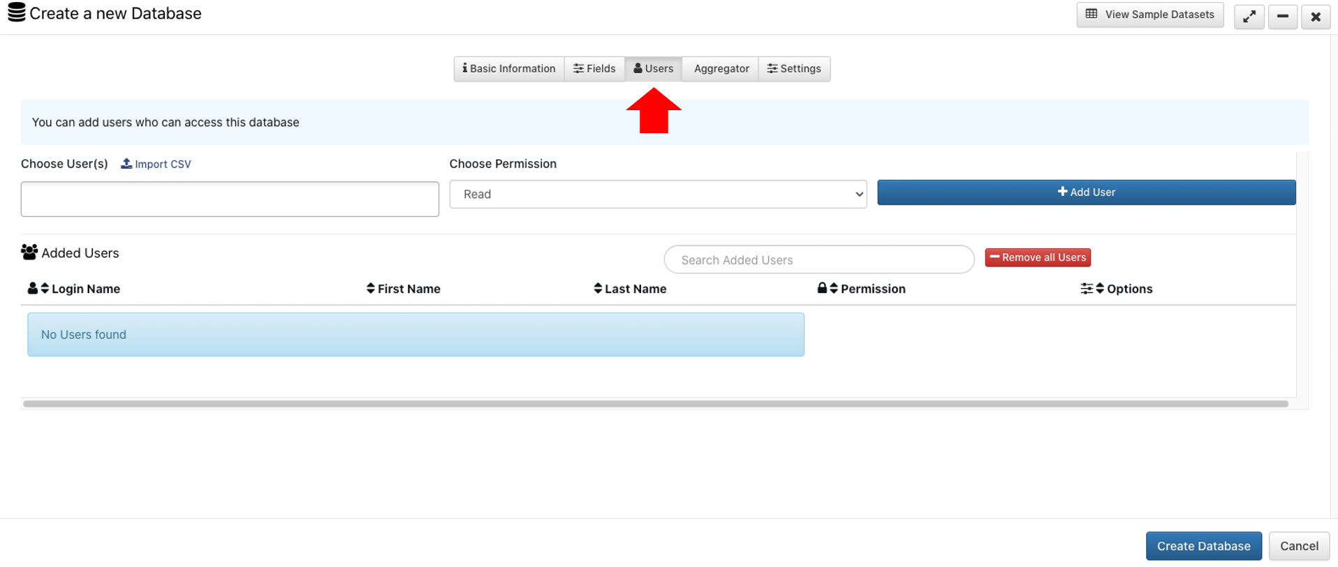
Step 3c. Add Users
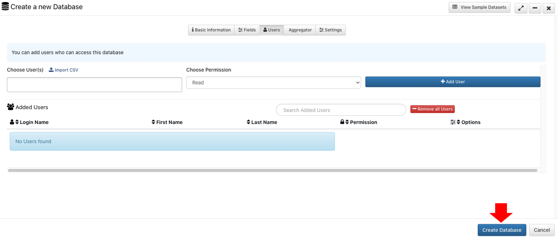
Step 3d. Save
Step 4. The New Database is now created. Click on the Name to open
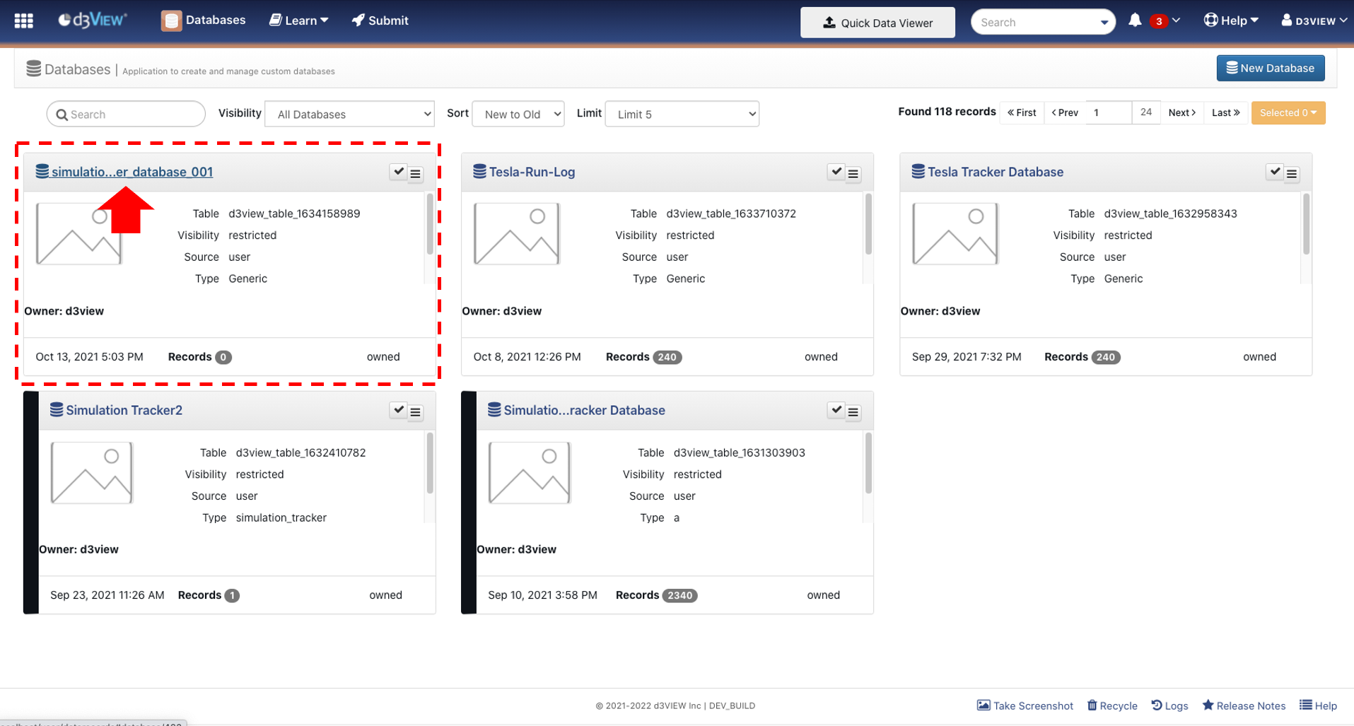
Step 5. Click ‘Add Record’ to add entry to the database
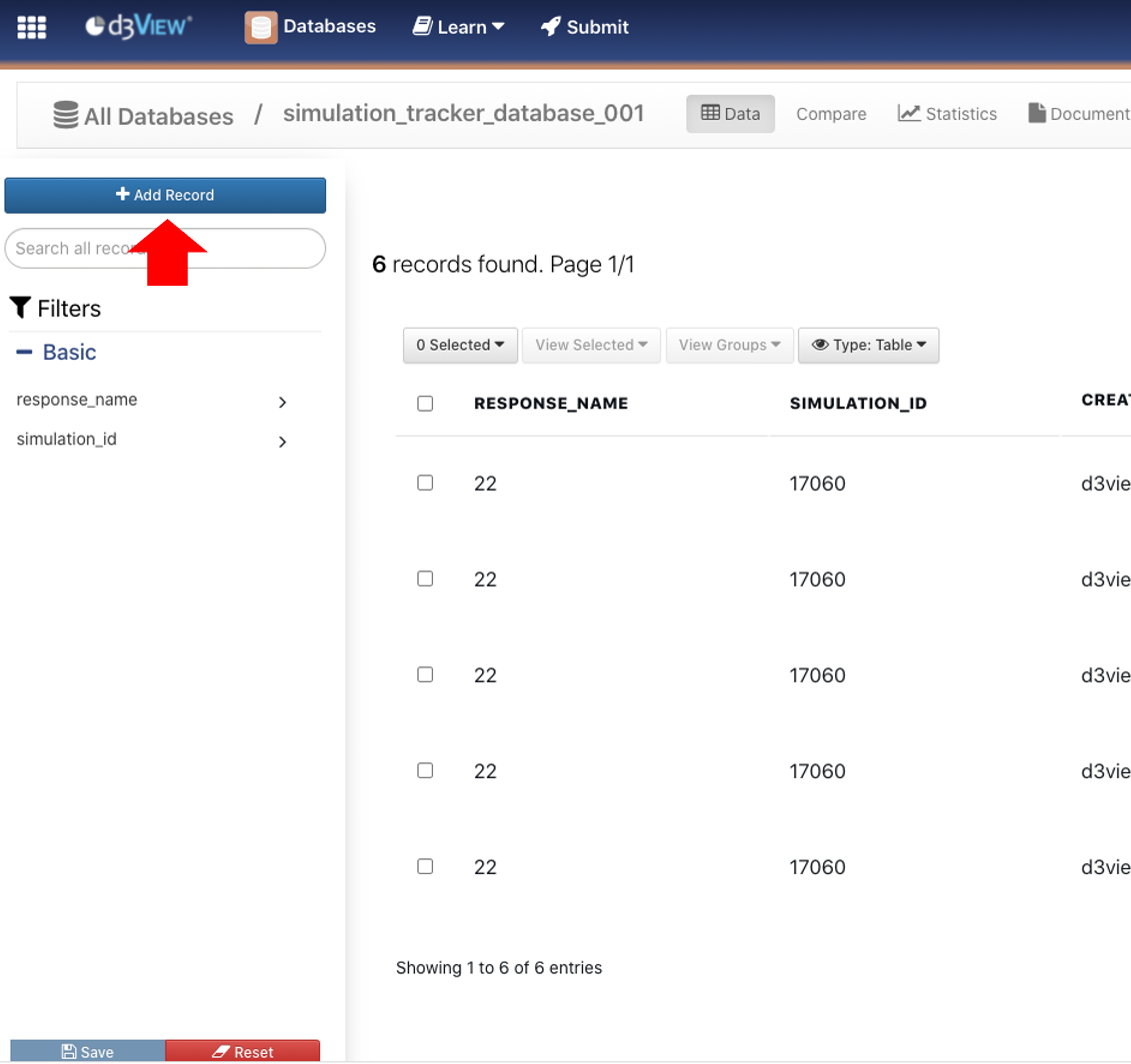
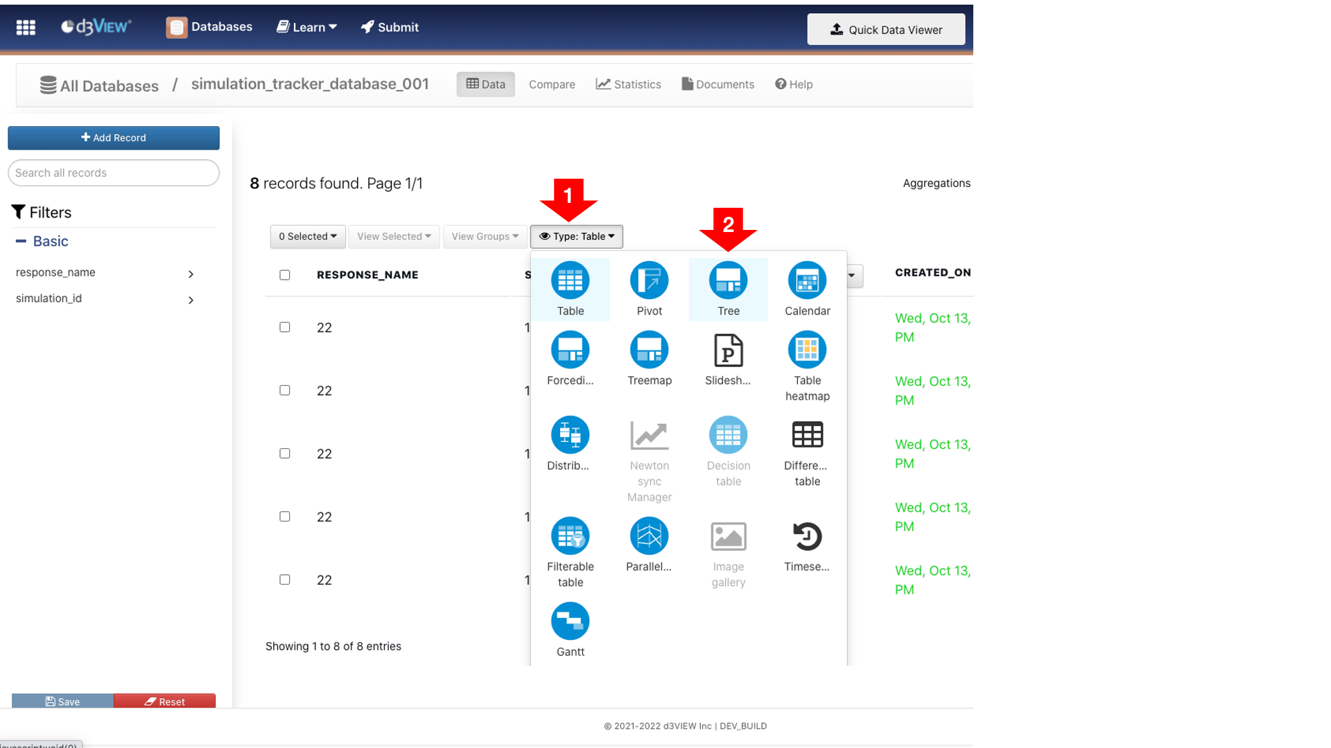
Last Step. Visualize records
Option C
For this option, we’ll create a database in d3VIEW and insert from a simulation or use a worker to populate the database as shown in the following image. (This requires simulations to be run and responses be available in d3VIEW).
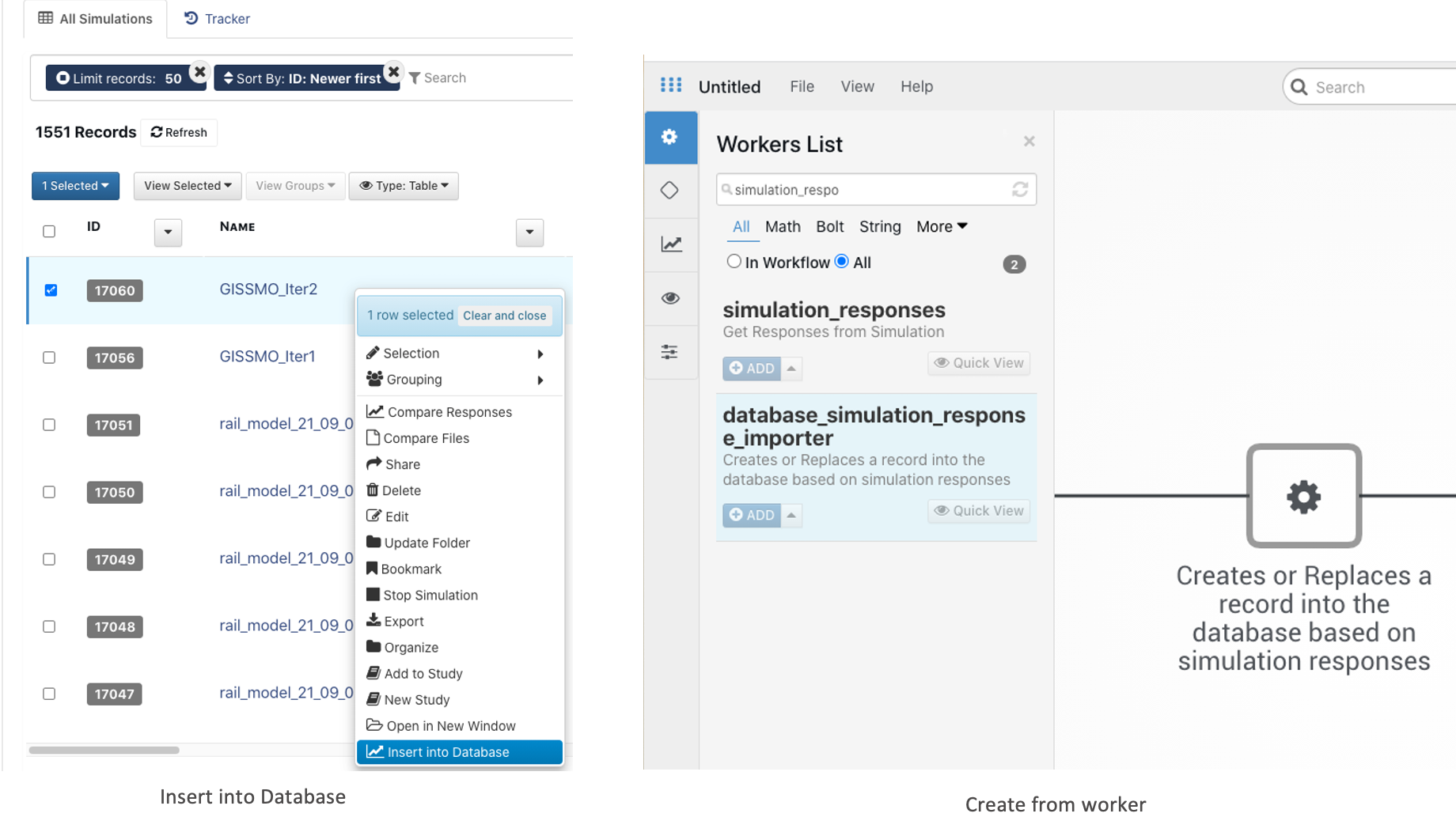
Figure 3: Option C: Insert from a simulation or using a Worker
6.12. Simulation Sharing
NEW as of March 21, 2022: There is added support to share records with selected teammates.
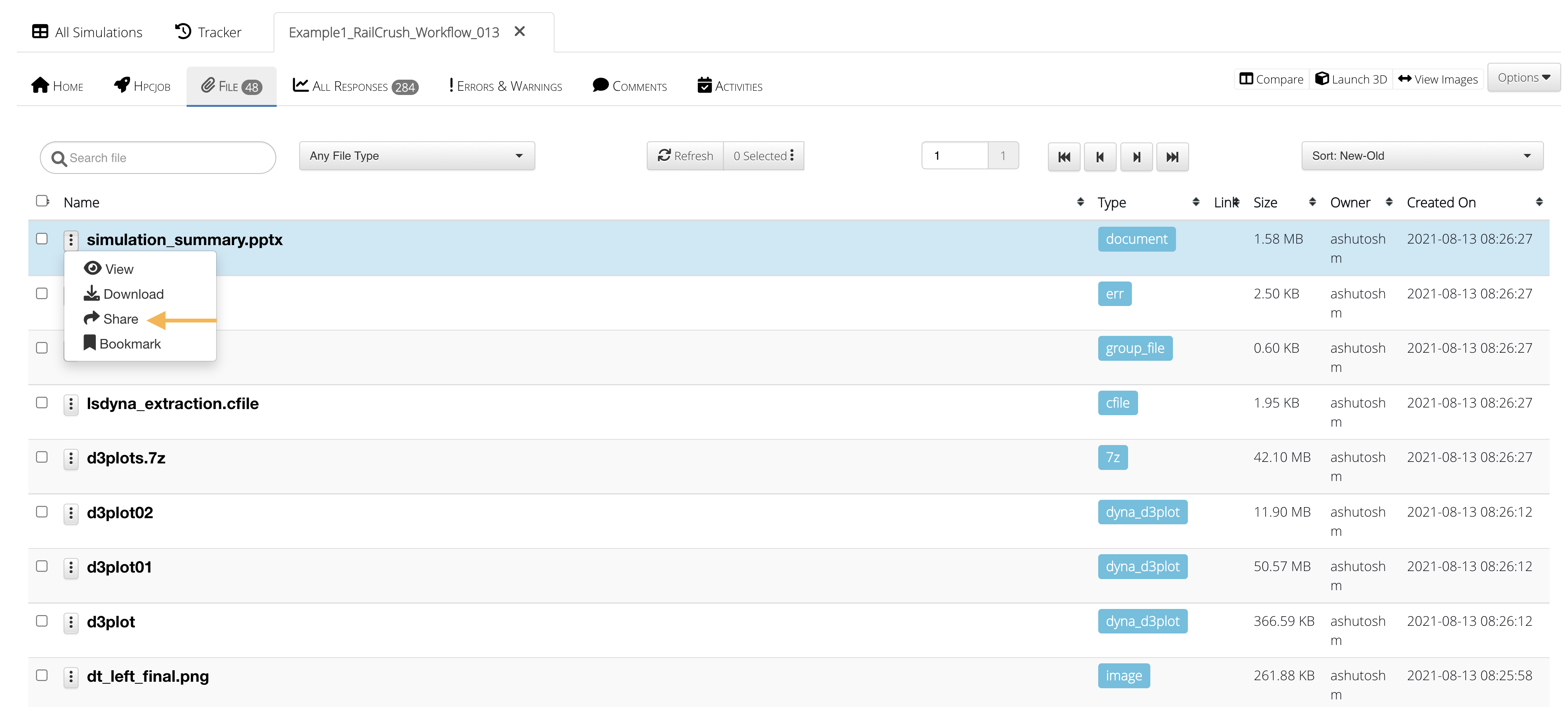
Figure 1: Share Simulation Records
There is also support to share a public link to anyone even those who do not have a d3VIEW account.
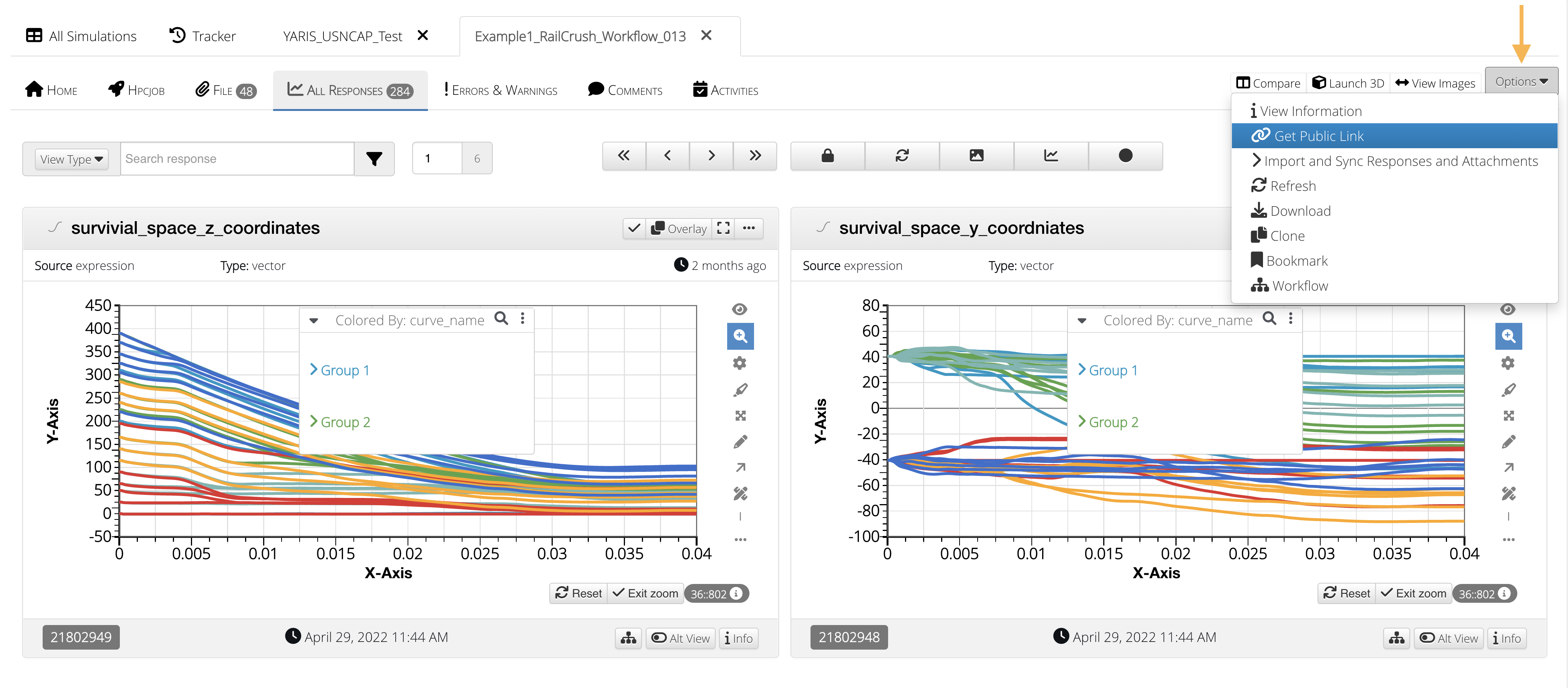
Figure 2: Share Public Simulation Link
6.13. Simulation Comments
Under the Comments tab, add any important notes about the simulation. This is especially useful for team communication. As of March 19, 2022, you can now directly tag other d3VIEW users on your team as well as tag simulation IDs in a comment.
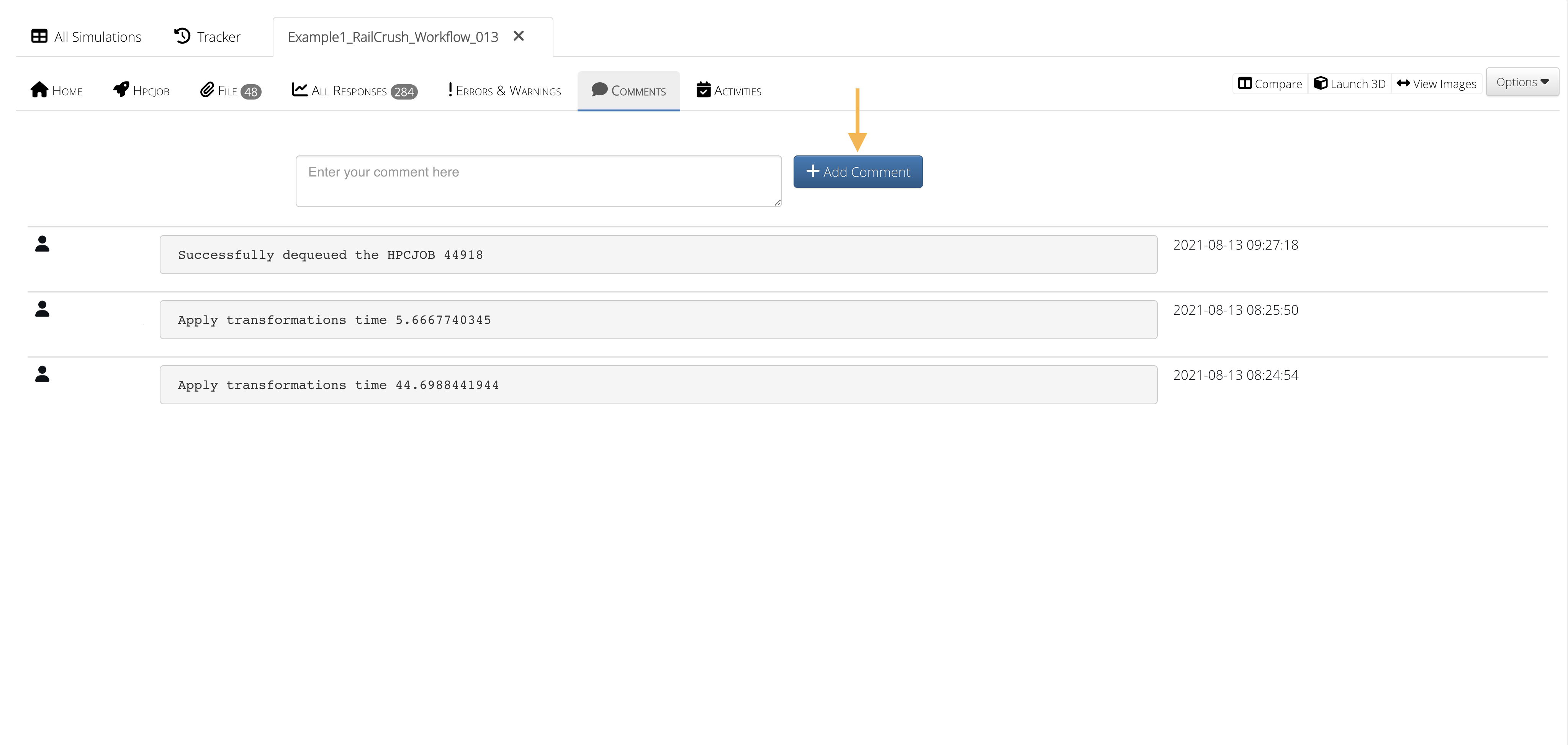
Figure 1: Simulation Comments
6.14. Simulation filters
Physical tests/Simulations can now be ordered randomly using filters.
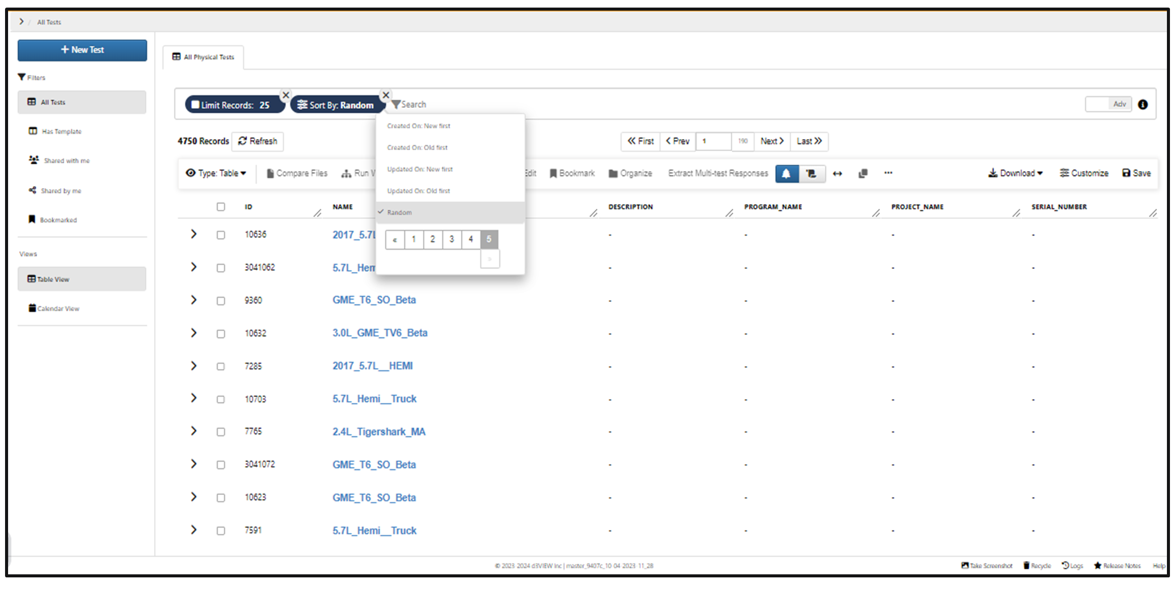
Random
In Simulations page, the horizontal scroll bar is available for filters when multiple filters are added to the list.
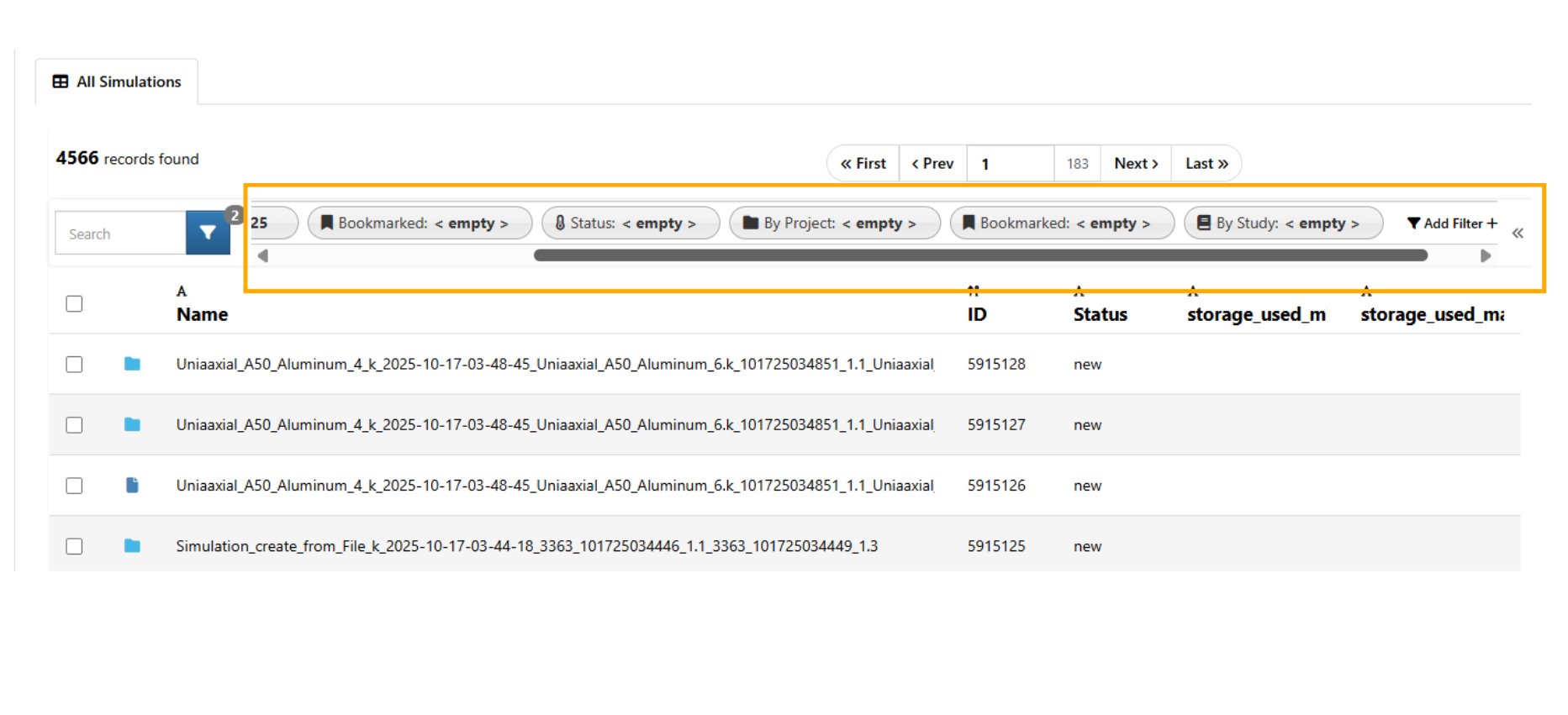
Filters scroll
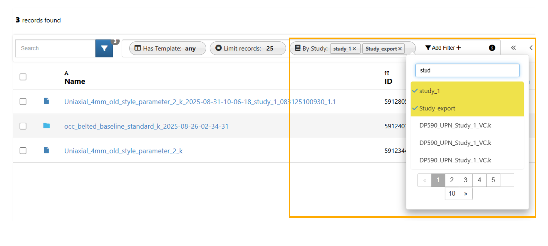
Added option in filters to allow filtering simulations by studies, with support for selecting multiple studies.
Simulations by studies
In Simulation, ‘By System Model’ and ‘By Assembly’ options are added as filters.

By System Model and By Assembly
6.15. Join Split Files
New option available under each simulation in the menu list to Join split files.
New tab
Workflows/ Physicaltests/ Simulations can now re-opened in a new tab from option available in the context menu.
For additional questions about how to navigate the d3VIEW platform, please feel free to email our team at: support@d3view.com.
6.16. Nested Context menu
New nested context menu options are available for the simulation records in Submit HPC feature in Simulations page.
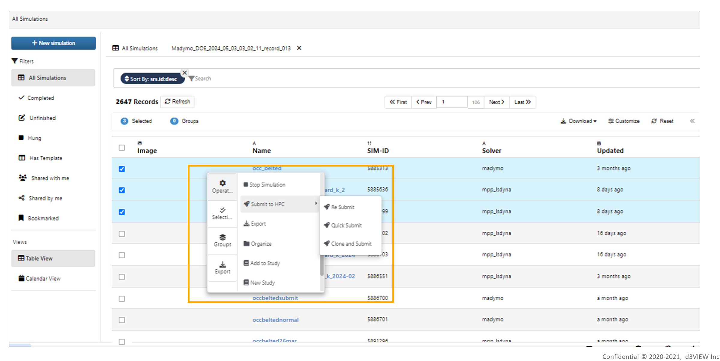
Nested Context Menu
6.17. Parent child
New option called ‘Enable parent/child view’ is available under preferences for Datatable records.
6.18. Datatable
A new DataTable UI is now available across the d3VIEW platform, featuring updated filter buttons and improved selection options.
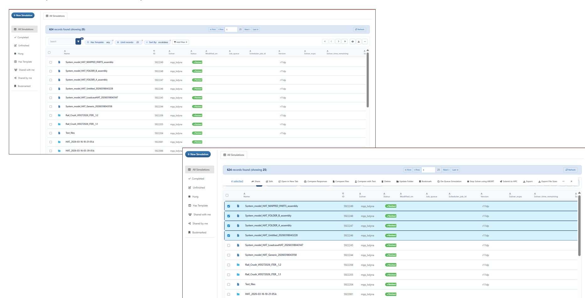
Datatable
Detailed view
The Datatable header now contains a View dropdown which will allow the user to choose between Detailed view or Default view.
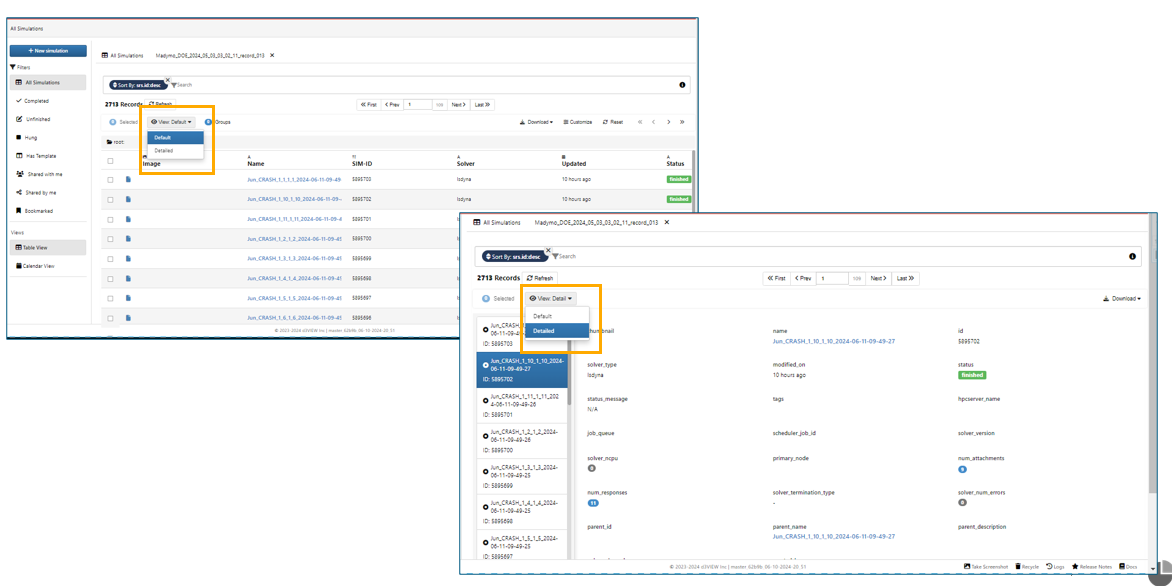
Detailed view
In Datatable, the detailed view has been updated to support expand/collapse nodes for parent simulations that contain child simulations.
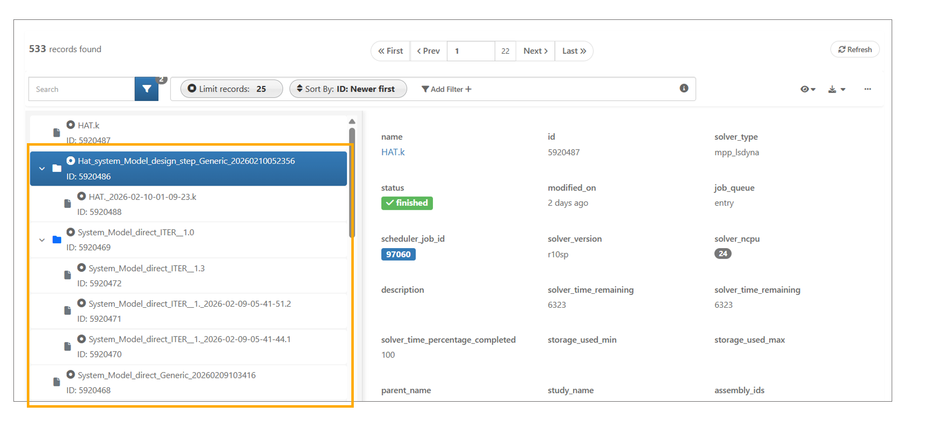
Detailed view
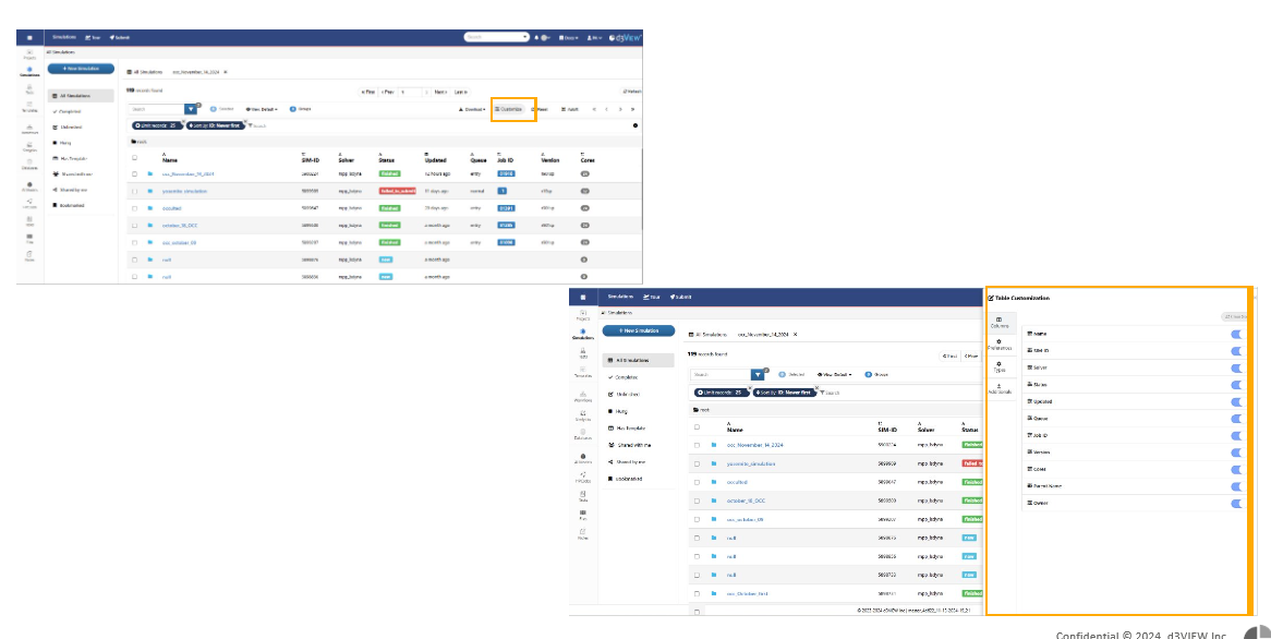
The new Table Viewer has option to show/toggle columns on the fly in the Customize sidebar.
Toggle columns
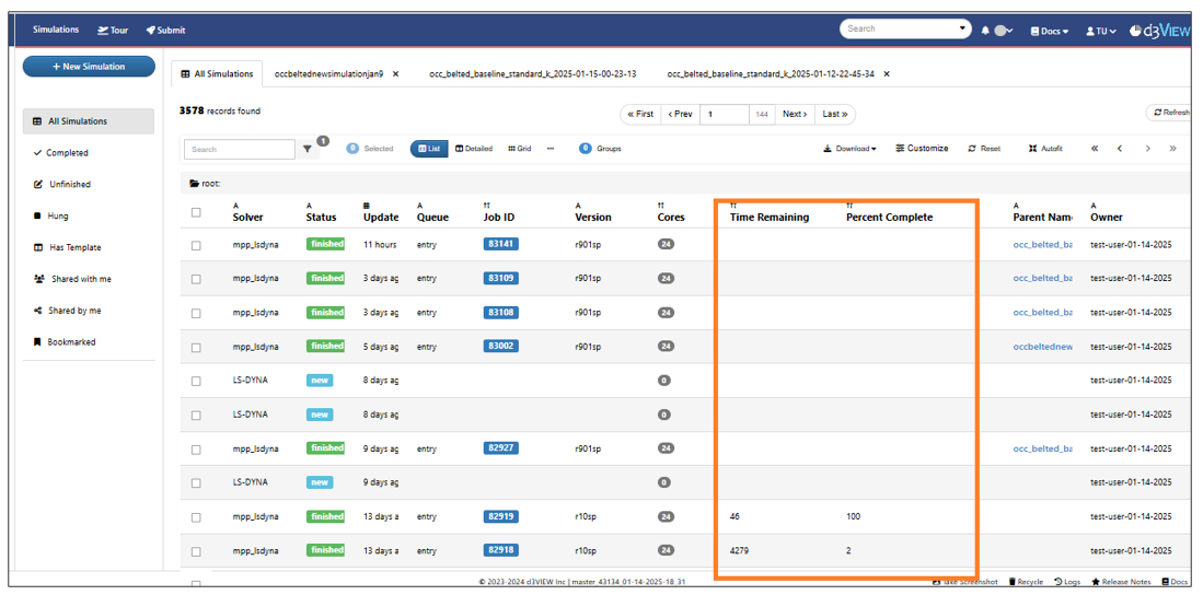
Simulation data table has two new columns called ‘Time Remaining and Percent Complete’ for the simulation records.
Time Remaining and Percent Complete
Simulations page now contains Assembly IDs and SystemModel IDs columns
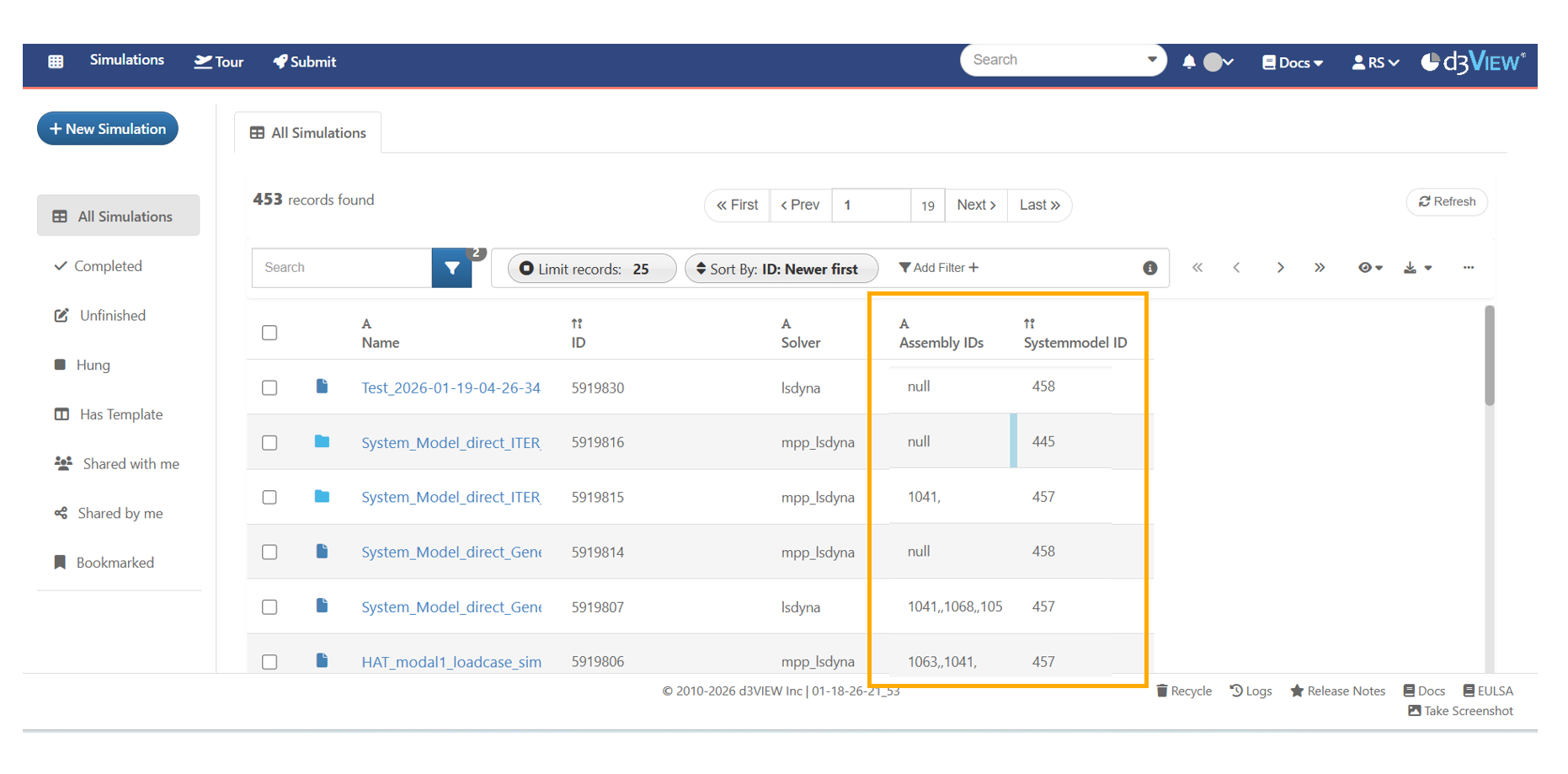
Assembly IDs and SystemModel IDs
Header Breadcrumbs
Datatable header will now show root breadcrumbs only when double clicked on folder icon of the records.
6.19. Additionals
New option called Additionals is added to the Datatable customize option, which will add/replace new columns to the records based on selection of records and template.
6.20. Filters
New integrated filters view is available for Datatables across the platform.
Reset option in Datatable now resets the non-default filters in the page.
6.21. Edit
Edit simulations now can support filter based selections for Project/Workflows/Templates.

filter based selections
Workflows can now be edited in the Simulation edit window.
In Multiple Edit window of a Homepage Data table, we have a Reset button in the Options column to reset values of the row.
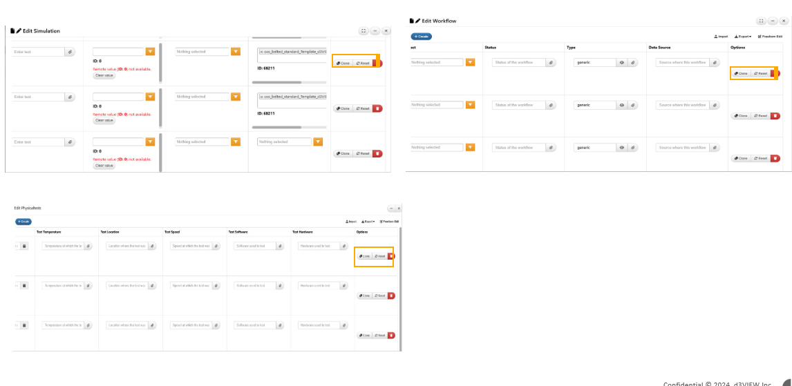
Multiple Edit
In Homepage Data table, we can select the header columns to view context menu options for - Clear selections and Compare.
6.22. Recycled Bin
Simulation records moved into Recycle bin upon deletion can be viewed and restored
Recycled items/records can be deleted from the recycled bin.
Number of records deleted from the recycled bin are showed on the screen.
6.23. Clear Up Space by deleting files
Deleting a Simulation
We can delete the Simulation using context menu options
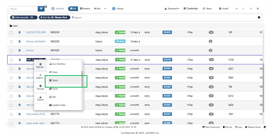
Delete the Simulation
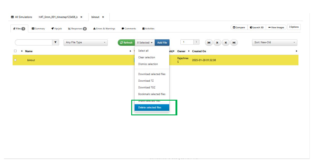
Deleting a File in Simulation
Files can be selected and deleted using option available in the header. These files will be permanently deleted from the simulation
Delete File
Recycled Bin
We can find all the deleted file in the Recycled bin available in the bottom of the page
Recycled Bin
Recycled bin shows deleted records based on the type of the record; we can check the deleted records for each type.
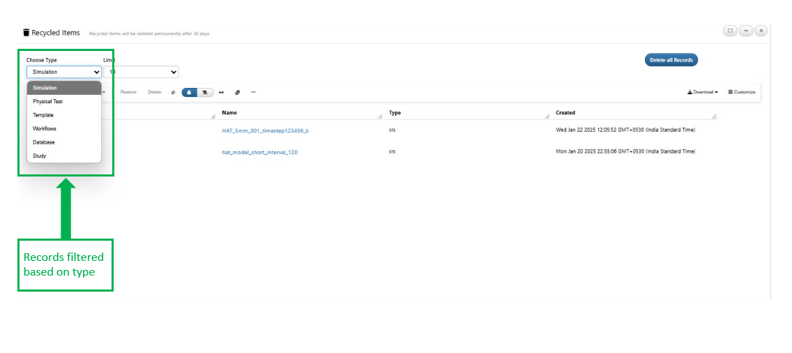
Type of Records
The records in the ‘Recycled Bin’ can be deleted or restored back based on type using the context menu options
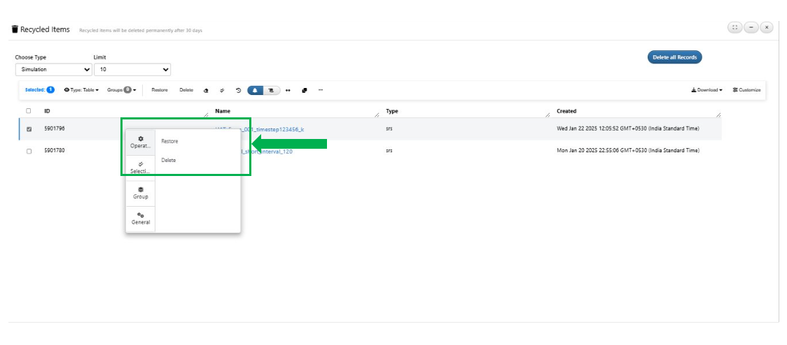
Delete restore
The space can be cleared by deleting all the records from the Recycled Bin
The option ‘Delete all records’ is available to delete and records and to clear the space
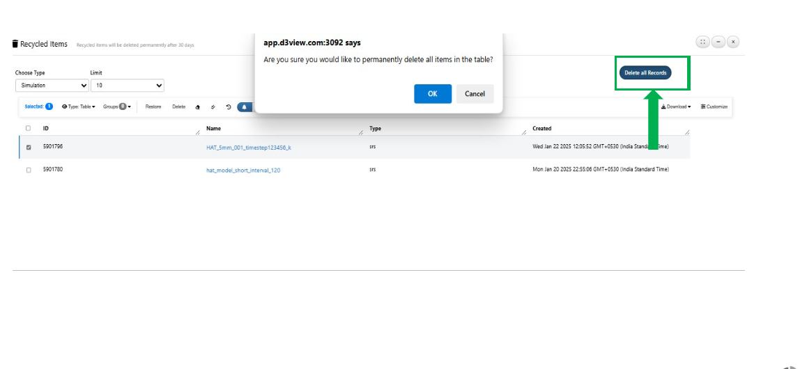
Delete all records
6.24. Comparision of Simulation with Physical test
New option is available in the context menu of the Simulation to compare the Simulation responses with Physical test responses in Simlytiks.
Video below shows how to compare simulation with Physical test.
Comparison of simulation with physical test has options for responses called quantities and scale factors. The quantities are auto detected when a test is selected, and the scale factors are updated corresponding to the quantities.
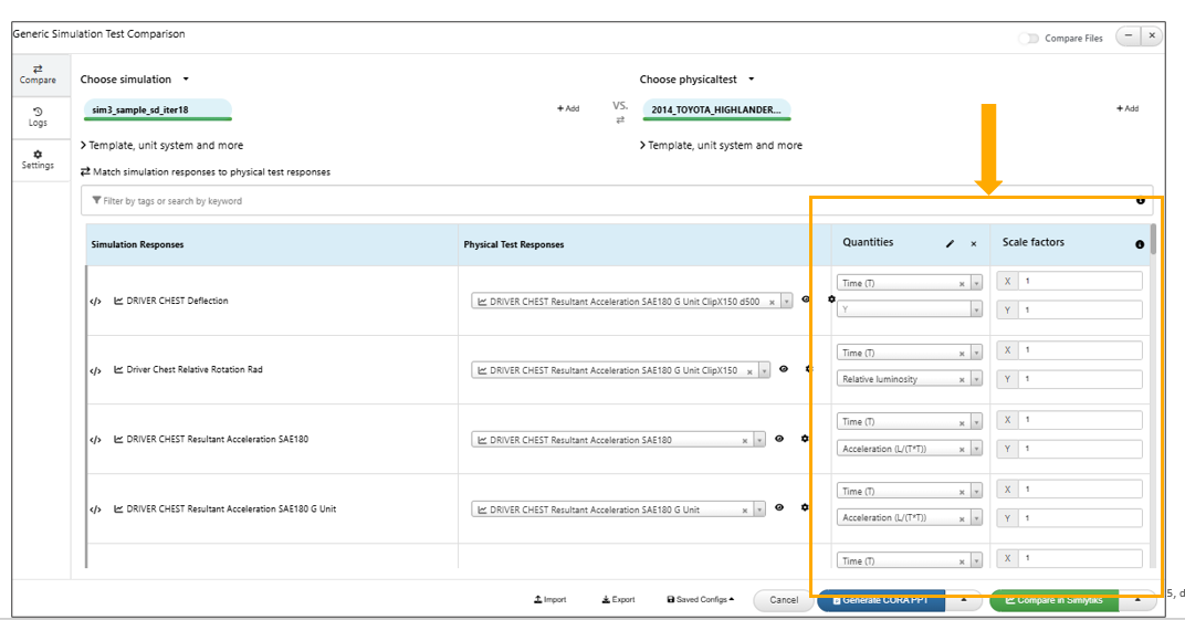
quantities and scale factors
Simulation to physical test comparison supports application of template, usage of template layout and ability to choose unit system.
In Simulation to physical test comparison, the names of the simulation, color and thickness for the curves in the responses can be modified and saved. These changes will be saved and observed in simlytiks after comparison.
Multiple records can be selected in simulation or physical test in simulation to physical test compare modal.
Comparison of simulation with physical test responses configurations can be exported, imported and saved to the modal.
In Simulation to physical test comparison, new options such as create one response per page, select view, one pager, sort responses order and selection of 3rd unit system are available in ‘Compare in Simlytiks’ button.
The Simlytiks page after comparing simulation to physical test will have two options, one is to generate the PPT for the pages and visualizations created and the other one is to go back to Sim/test comparison modal.
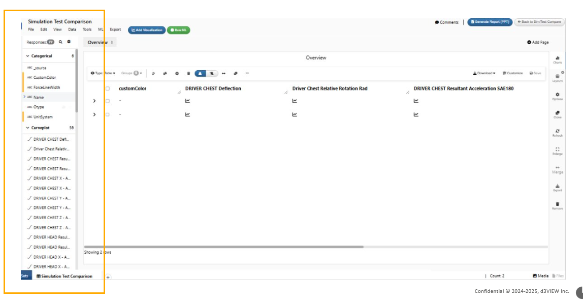
The Simlytiks responses are grouped based on the category while comparing simulation to physical test responses.
grouped based on the category
All physical test responses will now show a settings button on the right side of the response, which allows the user to add curve operations to the response.
The response name from the simulations can be clicked to view the response and we have eye icon to view the physical test responses in simulation to test comparison modal.
Export as CSV
Simulations to Physical test comparison now supports exporting the mapping data in the CSV format. This data can then be edited in the CSV file to update any mapping and imported back into the comparison modal.
Side by side view
Simulation to Physical test comparison now has a new view type called side by side view under settings option in modal
Finding closest Physical test
New option called ‘Finding closest test using workflow’ is available while comparing simulation to physical test. This option allows the user to execute the workflow and get the closest physical test from the multiple tests selected for comparison.
6.25. Simulation to Simlytiks compare
Simulation to physical test comparison will now support comparison of simulation responses with Simlytiks dataset by rows and responses.
Compare feature is now available in the footer options after selecting the records by highlighting them in Simlytiks visualizations.
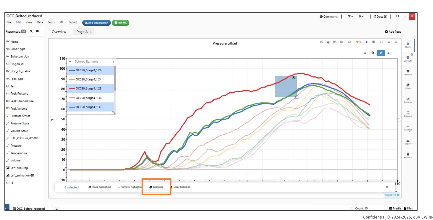
Compare
Multiple Simulations can be compared with Simlytiks dataset using the ‘Compare with Test’ option along with the template.
6.26. Organize
Studies can be now selected for Physical tests and Simulations in the Organize option.
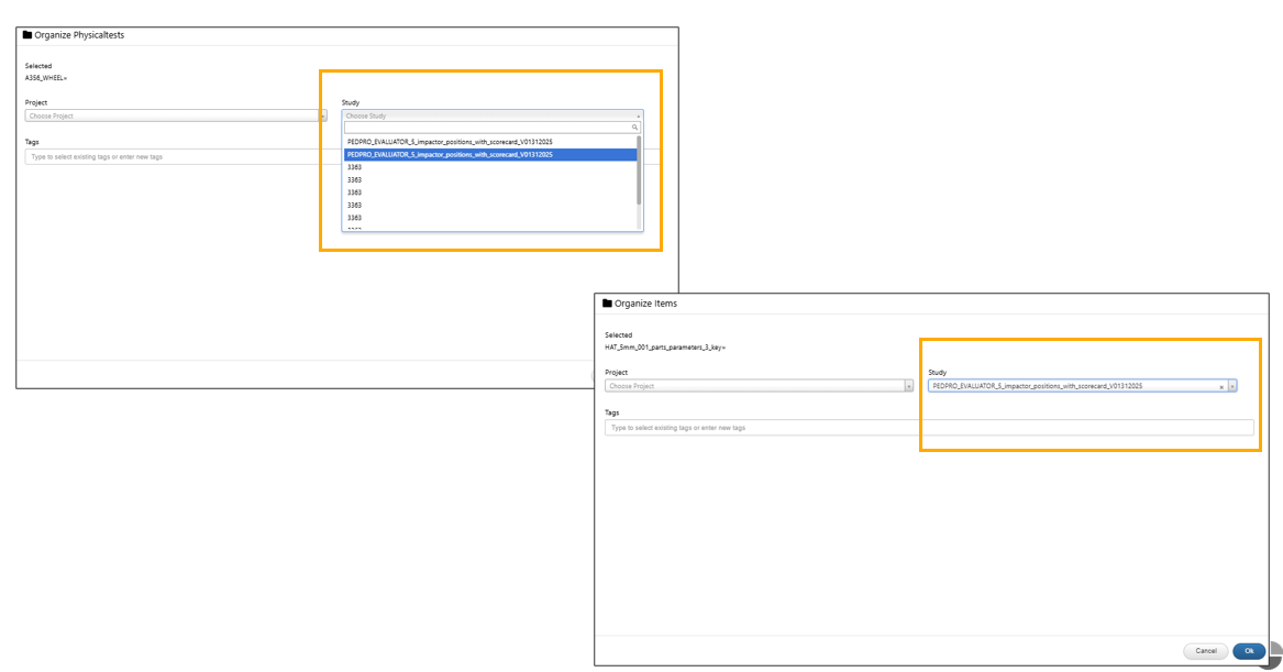
Organize
6.27. Multiselect
Resizing of the multiselect tab is now supported in the extract responses page
Multiselect tab in create response page now has a new setting in the sliders dropdown to show count for the list of items.
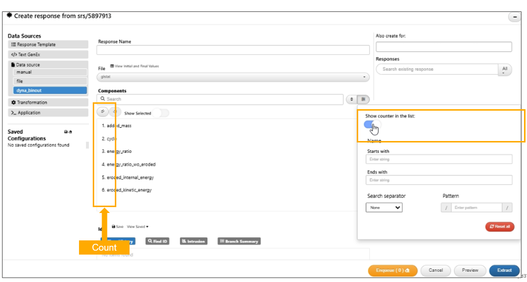
Show count for the list
Multi-Select has options such as ‘Select All’ , ‘Clear All Selections’ and ‘Show Selected’. The options selected here can be viewed in enlarged mode.
Export as Workflows
Simulation responses can now be exported using “Export as Wokflow” option to a workflow. The exported workflow can then be imported as a new workflow where the START worker will have the curve inputsfrom the exported responses.
6.28. Binout Visualization
Binout visualization with sparklines are created for the initial and final values when we click on ‘View initial/final’ values for binout table in response extraction.
Filters and search is now available for smooth filtering of the binout table in binout visualization with sparklines.
Settings is now available to toggle Sparkline Matrix with values in view initial and final values binout table.
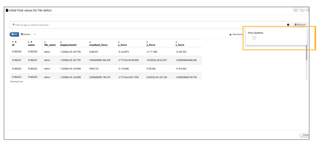
Sparkline Matrix with values
Clicking on the name in the Binout visualization will now show details in sidebar.
In Binout table , standalone Graphr is opened when we click on sparklines. The responses/sparklines will append to the containers in the GraphR application when we open them.
View 3D
Nodout file in Binout table has a View 3D button which renders the coordinates with colors in 3d scatter plot.
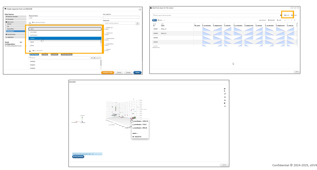
View 3D
In Binout table, viewing 3D for nodout data is now a 3-step process 1) Points to be selected in 3D Scatter view. 2) Show labels in 3D Scatter above the circles as labelBy and 3) Choose components in 2nd step which when applied sends all the responses to Graphr.
6.29. Text Difference
We now have the option to view the text difference between 2 simulation response files upon comparison in Simlytiks.
New option is added in Text difference checker called ‘case sensitiveness’ which helps user in searching case sensitive keywords in the files while comparing simulation files.
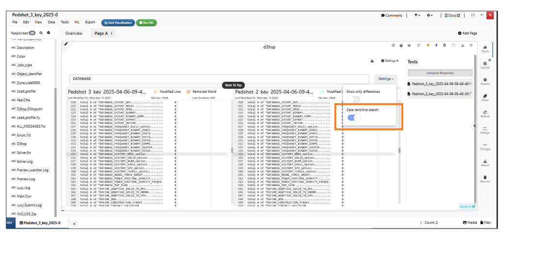
Case sensitiveness
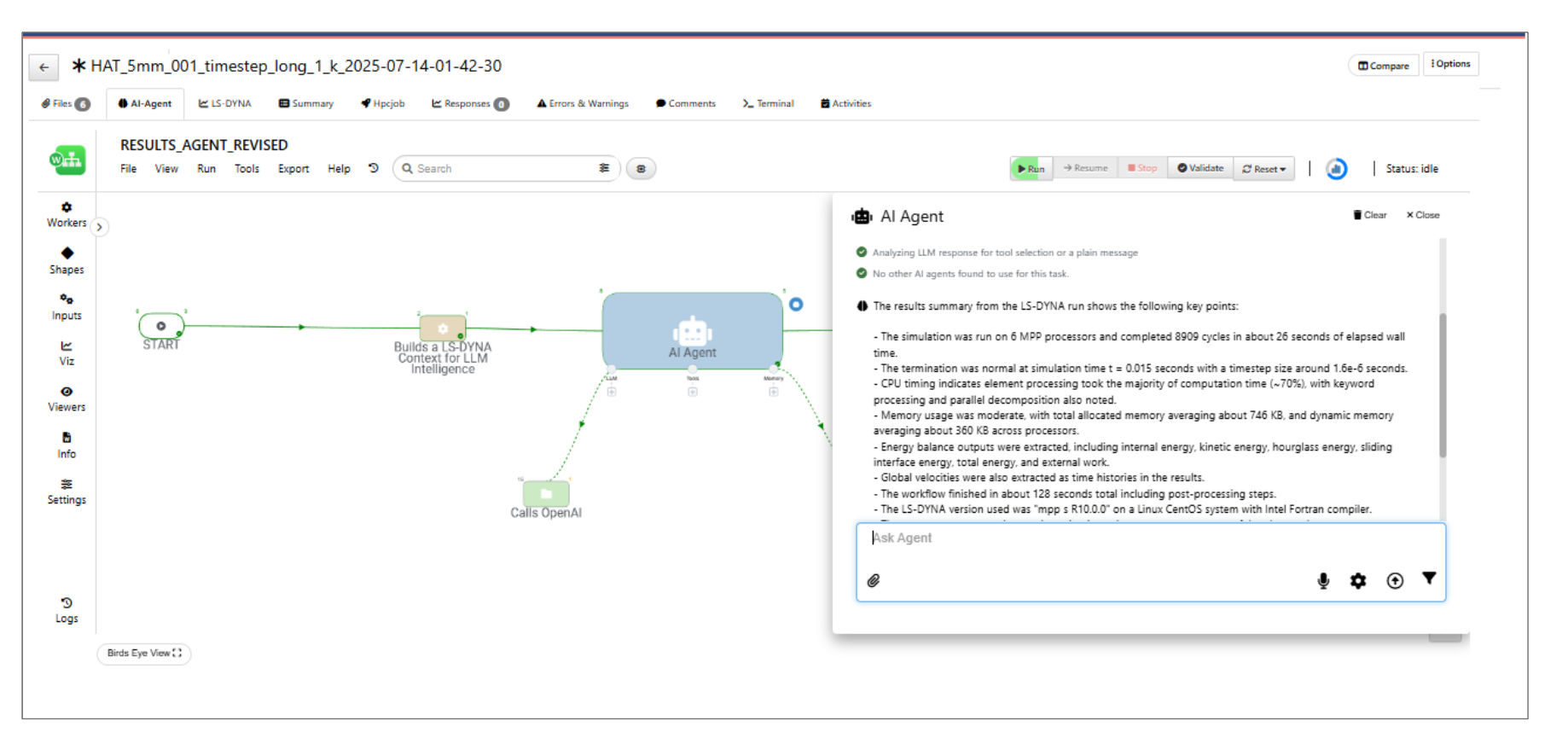
6.32. AI Agent
The AI_Agent tab within a simulation will execute the AI Agent worker and display the simulation summary results in the prompt.
Terminal
6.33. BOM Columns
The BOM option is now visible when hovering over a simulation name in the Simulation page , which shows the BOM graph view of the Simulation.
In the SIMULATION module, an error message is now displayed when no GRAPH information is available for a simulation.
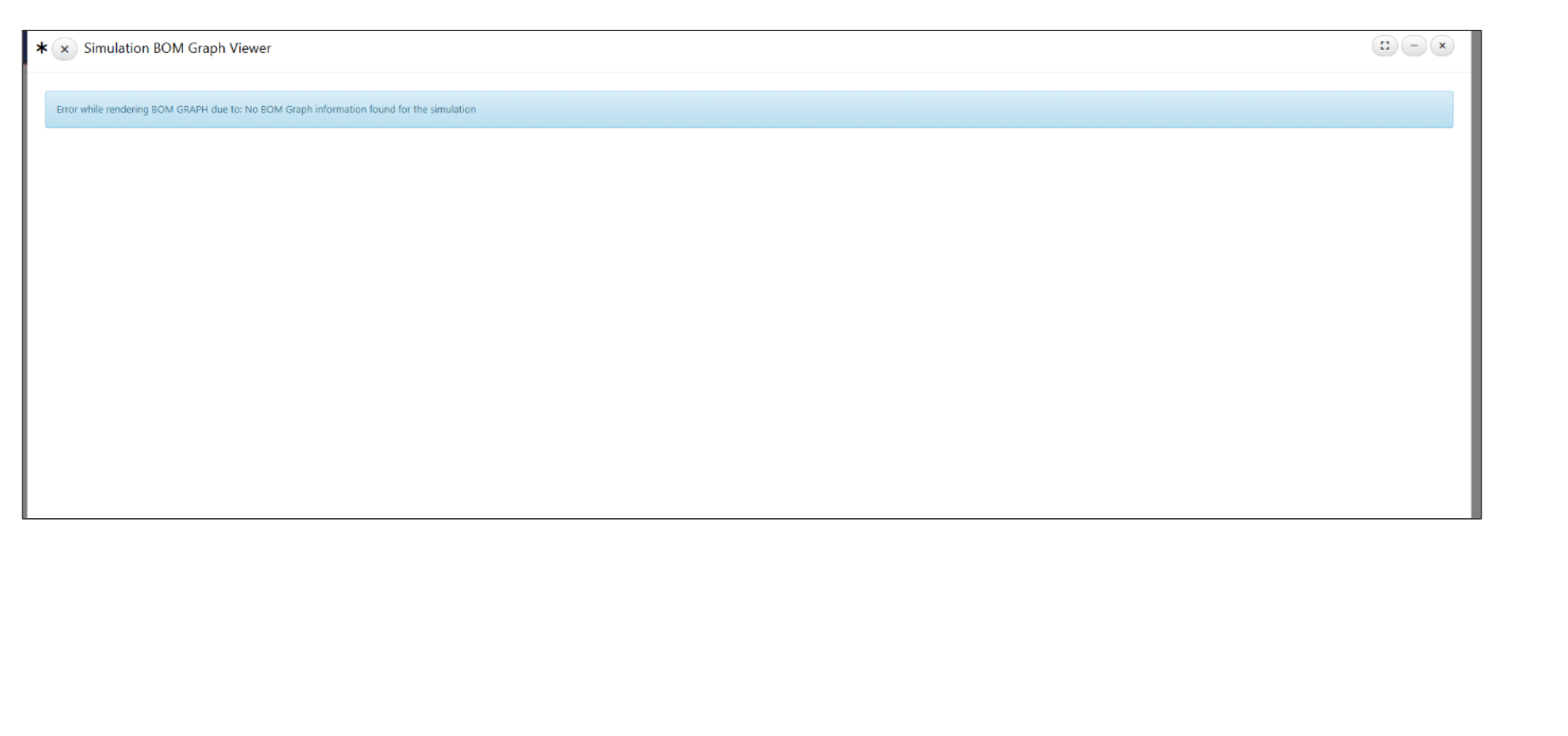
BOM Columns
6.34. Files and Responses
In the Simulation module, you can now view responses and attached files directly from each simulation row in the simulation table.
6.35. Operations
Newton responses from Simulations/Physicaltests can be operated using context menu options. The operated curve will replace the existing curve in the response and can be reverted back to the original curve using the context menu options.
6.36. Configure template
Template can be configured while submitting a Simulation. This configured template details will be saved in the simulation files page as a .d3pptd file.
New option called ‘Export File Sizes’ is available in the header options for simulation records.
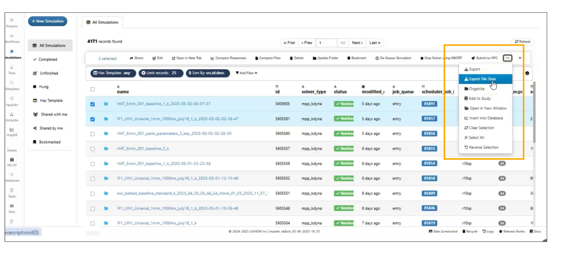
Export File Sizes
6.37. Result Explorer with AI
Right context menu of a Simulation has a new option called ‘Result Explorer with AI’.
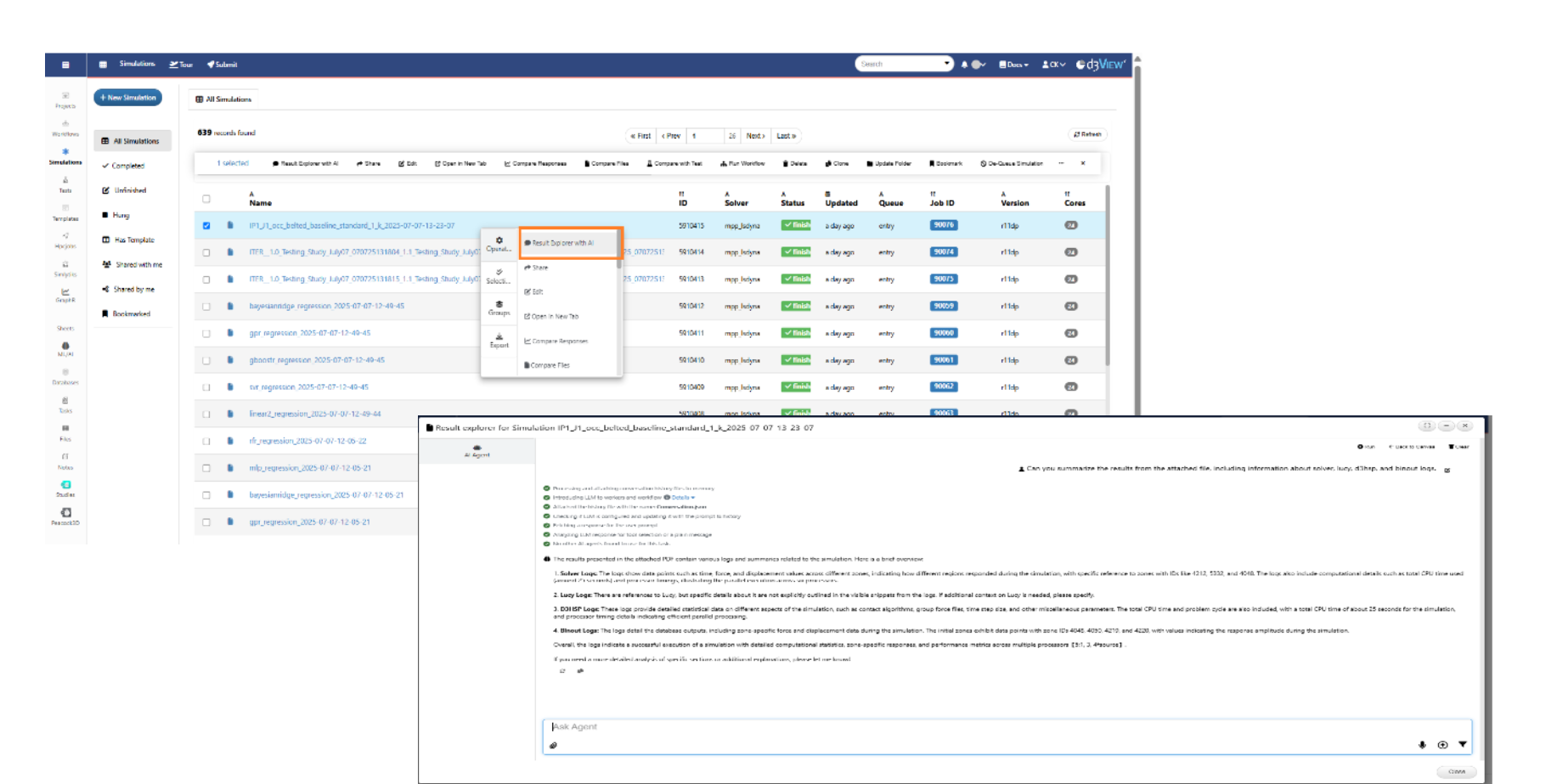
Result Explorer with AI
6.38. New Submit
Updated the Try New Submit and Classic buttons with an orange-themed style.
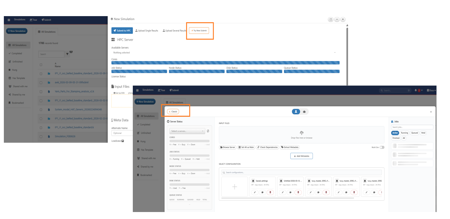
Try New Submit
New Submit Window: Added toggle-deselect functionality that allows users to deselect saved configuration cards by clicking on them again.
New Submit Modal: Revamped the submit modal to include a version toggle and server status display.
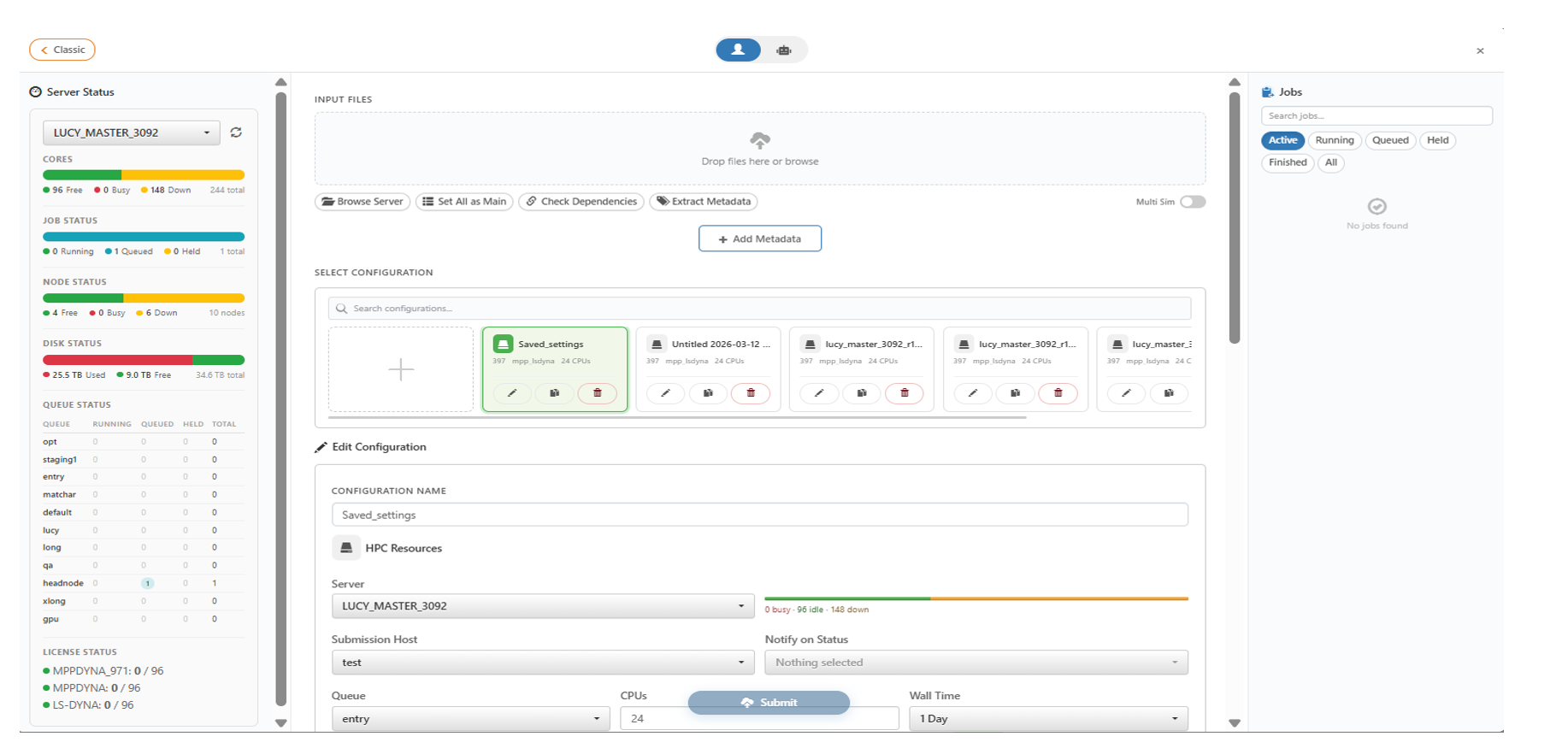
Version toggle and server status display