
6.  Examples
6.1. Workflow Collection
| Name | ID | Description |
|---|---|---|
| Engstressstrain_to_MAT | 004 | Converts stress-strain curve to Material card MAT 024 |
| MATERIAL_VARIANCE | 005 | Converts variance curves for MAT_024 using min/mean/max |
| Steel_Casting_Polymer_StressStrain_to_MAT24 | 006 | Converts Eng-stress-strain curve with custom post necking treatment |
| HIC_ML_AUTO_WORKFLOW | 007 | Uses ML_LEARN_AUTO to learn and predict from dataset. |
| GISSMO_regularization_Workflow | 008 | Helps calibrate the mesh-regularization scale factors for MAT_ADD_EROSION card |
| SPOTWELD_FAILURE_PREDITIONS | 009 | Using ORNL Spotweld Data, spotwelds failure can be predicted |
| LS-DYNA_Material_validator | 010 | Parses LS DYNA material data and validates the material curves and properties |
| Feature_Importance_Workflow | 011 | You can input the dataset and run feature importnace |
| DOE_DataAnalyzer | 012 | Generic Doe Analyzer Workflow |
| PolymerStrainRate_Workflow | 013 | Generic Polymer Calibration Workflow with Strain-rate effects. |
| Generic_Optimizer | 100 | With a Single input file, you can preform design sensitivity or optimize a structure |
| Time_history_learn/predict_G3_Workflow | 101 | Learns a Time history based on inputs and predicts it. |
| Post-necking_workflow | 103 | Post necking calibration for Metals. |
| GISSMO | 104 | GISSMO Material Calibration |
| NHTSA_Workflows | 105,106 | NHTSA based AI to predict Occupant rating based on vehicle information/cluster based on vehicle crassworthiness. |
| 200_BMS_PUBLISHER | 200 | Publishes BMS data into d3view |
| Madymo_sample_Workflow | 301 | Madymo basic DOE Workflow |
Sample Workflows are available in the Workflow collection Library. Below are the Workflows along with the links for the Sample Workflows available in the collection.
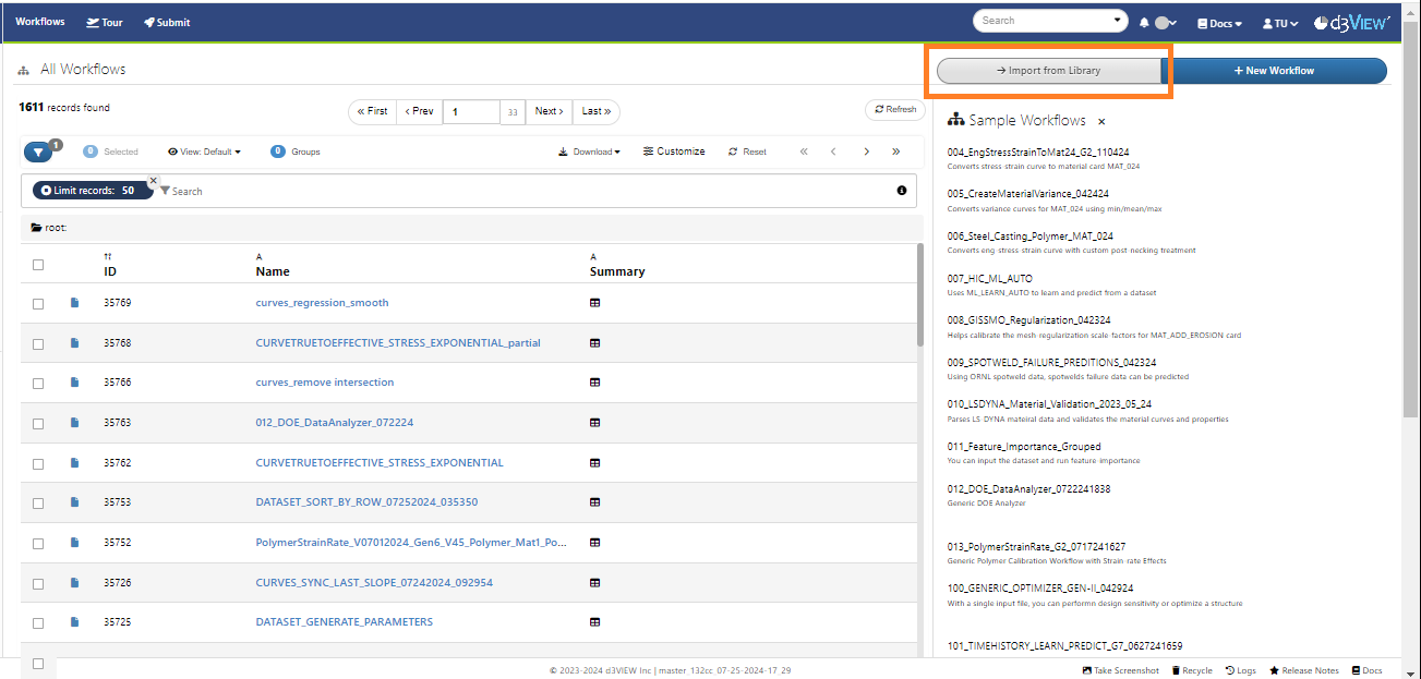
View workflow collection is now shifted to Files/library from tools.
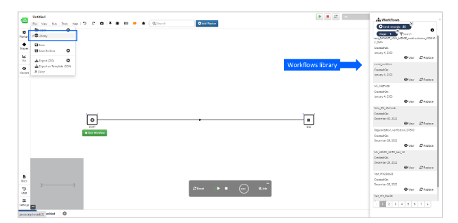
Figure 14: View Workflows collection
All library workflows are updated to ensure the files needed by the workflows are packaged. All workflows now should execute without an error about missing input files.
UI is updated for the Library option available under Files in Workflows
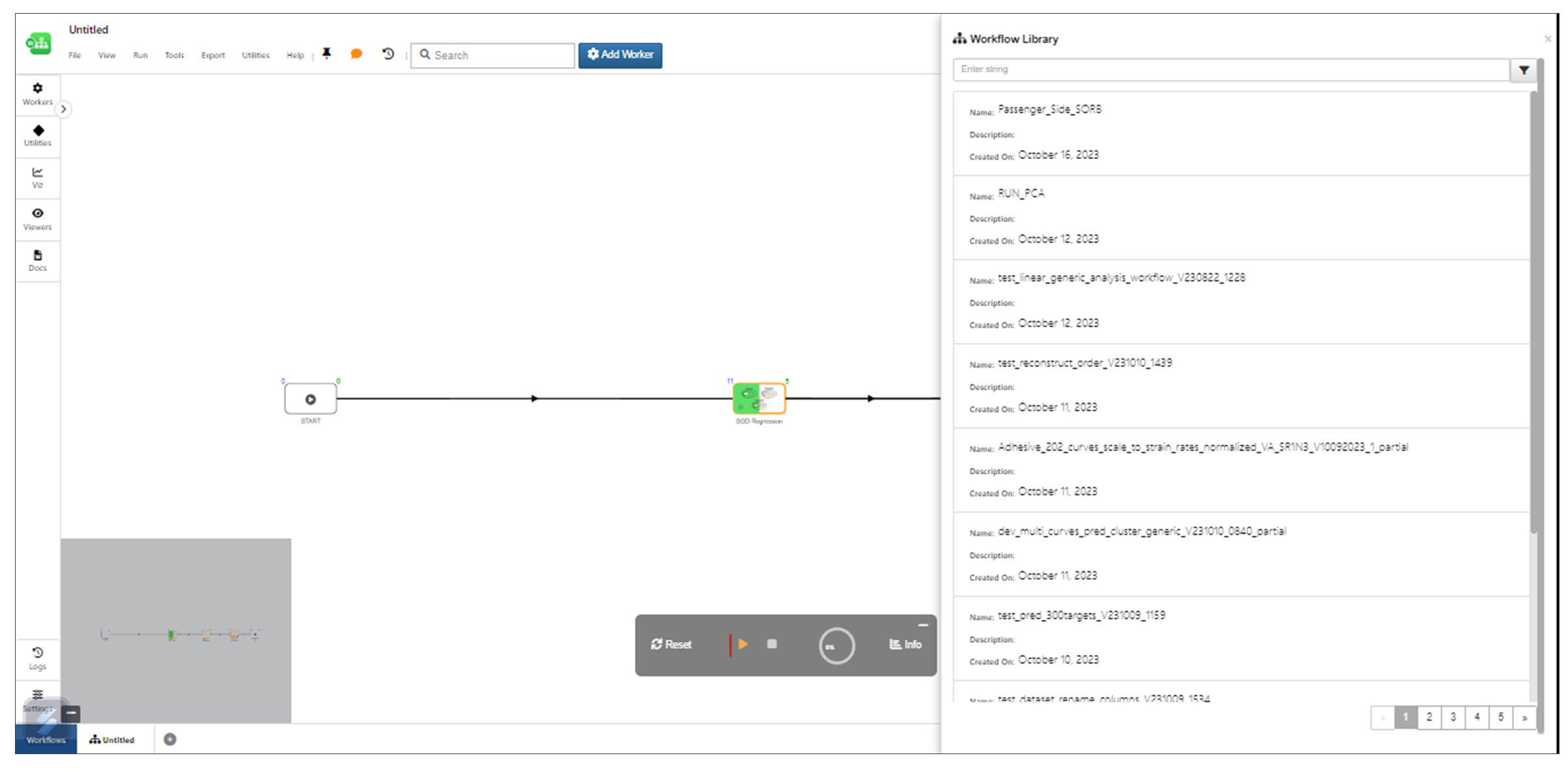
Library
6.2. Workflow Collection Videos
Few Library sample Workflows are associated with videos to show the execution of the Workflow with inputs.
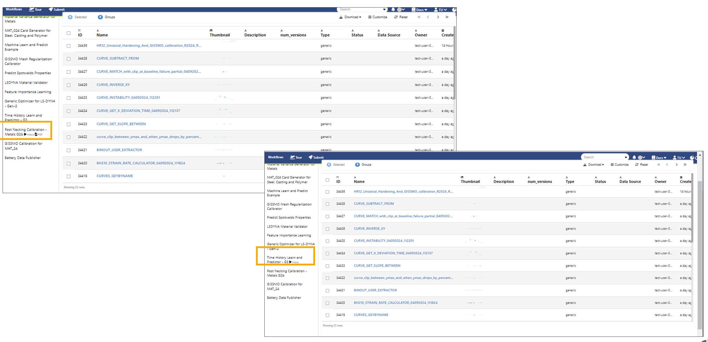
Workflow Video